TiDB Development Guide
![]()
About this guide
- The target audience of this guide is TiDB contributors, both new and experienced.
- The objective of this guide is to help contributors become an expert of TiDB, who is familiar with its design and implementation and thus is able to use it fluently in the real world as well as develop TiDB itself deeply.
The structure of this guide
At present, the guide is composed of the following parts:
- Get started: Setting up the development environment, build and connect to the tidb-server, the subsections are based on an imagined newbie user journey.
- Contribute to TiDB helps you quickly get involved in the TiDB community, which illustrates what contributions you can make and how to quickly make one.
- Understand TiDB: helps you to be familiar with basic distributed database concepts, build a knowledge base in your mind, including but not limited to SQL language, key components, algorithms in a distributed database. The audiences who are already familiar with these concepts can skip this section.
- Project Management: helps you to participate in team working, lead feature development, manage projects in the TiDB community.
Contributors ✨
Thanks goes to these wonderful people (emoji key):


This project follows the all-contributors specification. Contributions of any kind welcome!
Get Started
Let's start your TiDB journey! There's a lot to learn, but every journey starts somewhere. In this chapter, we'll discuss:
- Install Golang
- Get the code, build and run
- Setup an IDE
- Write and run unit tests
- Debug and profile
- Run and debug integration tests
- Commit code and submit a pull request
Install Golang
To build TiDB from source code, you need to install Go in your development environment first. If Go is not installed yet, you can follow the instructions in this document for installation.
Install Go
TiDB periodically upgrades its Go version to keep up with Golang. Currently, upgrade plans are announced on TiDB Internals forum.
To get the right version of Go, take a look at the go.mod file in TiDB's repository. You should see that there is a line like go 1.21 (the number may be different) in the first few lines of this file. You can also run the following command to get the Go version:
curl -s -S -L https://github.com/pingcap/tidb/blob/master/go.mod | grep -Eo "\"go [[:digit:]]+(\.[[:digit:]]+)+\""
Now that you've got the version number, go to Go's download page, choose the corresponding version, and then follow the installation instructions.
Manage the Go toolchain using gvm
If you are using Linux or MacOS, you can manage Go versions with Go Version Manager (gvm) easily.
To install gvm, run the following command:
curl -s -S -L https://raw.githubusercontent.com/moovweb/gvm/master/binscripts/gvm-installer | sh
Once you have gvm installed, you can use it to manage multiple different Go compilers with different versions. Let's install the corresponding Go version and set it as default:
TIDB_GOVERSION=$(curl -s -S -L https://github.com/pingcap/tidb/blob/master/go.mod | grep -Eo "\"go [[:digit:]]+(\.[[:digit:]]+)+\"" | grep -Eo "[[:digit:]]+\.[[:digit:]]+(\.[[:digit:]]+)?")
gvm install go${TIDB_GOVERSION}
gvm use go${TIDB_GOVERSION} --default
Now, you can type go version in the shell to verify the installation:
go version
# Note: In your case, the version number might not be '1.21', it should be the
#   same as the value of ${TIDB_GOVERSION}.
#
# OUTPUT:
# go version go1.21 linux/amd64
In the next chapter, you will learn how to obtain the TiDB source code and how to build it.
If you encounter any problems during your journey, do not hesitate to reach out on the TiDB Internals forum.
Get the code, build, and run
Prerequisites
git: The TiDB source code is hosted on GitHub as a git repository. To work with the git repository, please installgit.go: TiDB is a Go project. Therefore, you need a working Go environment to build it. See the previous Install Golang section to prepare the environment.gcc:gcccommand is required to usecgowhile building. To installgcc, search for appropriate install guide for your OS.mysqlclient (optional): After building TiDB from source, you can use the official MySQL client to connect to TiDB. It is not required if you want to build TiDB only.
Note:
TiDB could compile and run on Windows 10. However, it is not expected to be deployed on Windows, where you might encounter many compatibility problems. To have a better experience, we recommend you install WSL2 first.
Clone
Clone the source code to your development machine:
git clone https://github.com/pingcap/tidb.git
Build
Build TiDB from the source code:
cd tidb
make
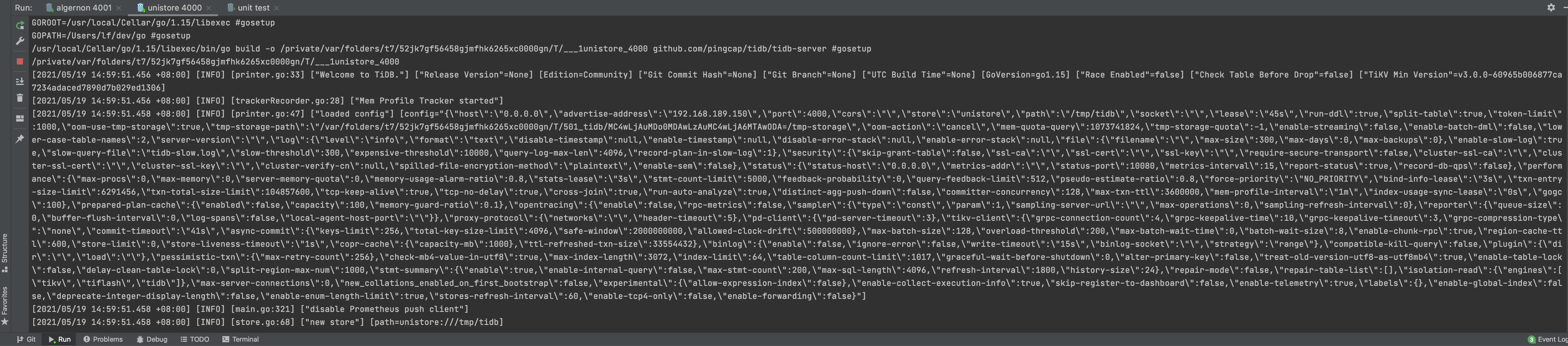
Run
Now that you have the tidb-server binary under the bin directory, execute it for a TiDB server instance:
./bin/tidb-server
This starts the TiDB server listening on port 4000 with embedded unistore.
Connect
You can use the official MySQL client to connect to TiDB:
mysql -h 127.0.0.1 -P 4000 -u root -D test --prompt="tidb> " --comments
where
-h 127.0.0.1sets the Host to local host loopback interface-P 4000uses port 4000-u rootconnects as root user (-pnot given; the development build has no password for root.)-D testuses the Schema/Database test--prompt "tidb> "sets the prompt to distinguish it from a connection to MySQL--commentspreserves comments like/*T
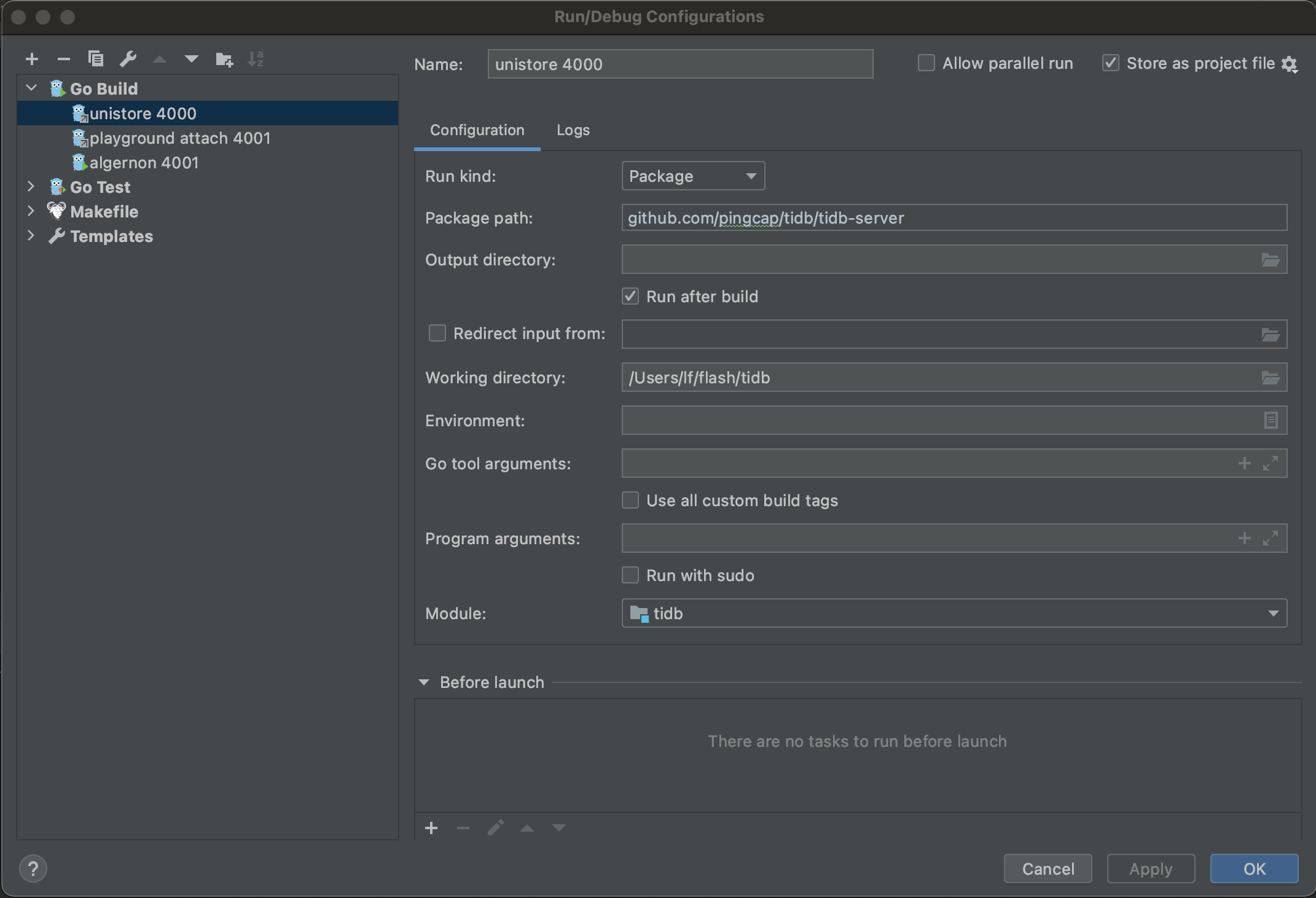
Populate run configurations
Under the root directory of the TiDB source code, execute the following commands to add config files:
mkdir -p .idea/runConfigurations/ && cd .idea/runConfigurations/
cat <<EOF > unistore_4000.xml
<component name="ProjectRunConfigurationManager">
<configuration default="false" name="unistore 4000" type="GoApplicationRunConfiguration" factoryName="Go Application">
<module name="tidb" />
<working_directory value="\$PROJECT_DIR\$" />
<kind value="PACKAGE" />
<filePath value="\$PROJECT_DIR\$" />
<package value="github.com/pingcap/tidb/cmd/tidb-server" />
<directory value="\$PROJECT_DIR\$" />
<method v="2" />
</configuration>
</component>
EOF
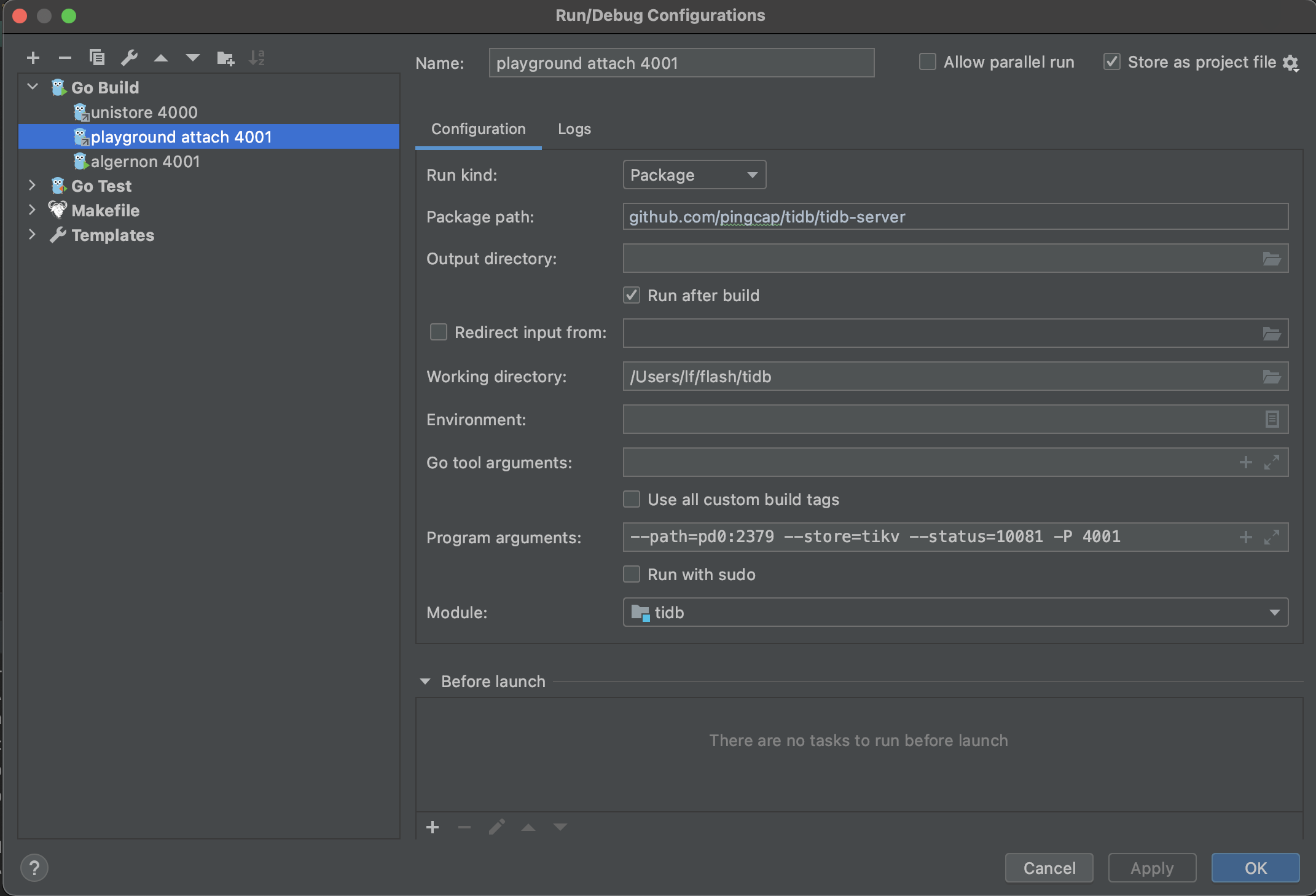
cat <<EOF > playground_attach_4001.xml
<component name="ProjectRunConfigurationManager">
<configuration default="false" name="playground attach 4001" type="GoApplicationRunConfiguration" factoryName="Go Application">
<module name="tidb" />
<working_directory value="\$PROJECT_DIR\$" />
<parameters value="--path=127.0.0.1:2379 --store=tikv --status=10081 -P 4001 " />
<kind value="PACKAGE" />
<filePath value="\$PROJECT_DIR\$/cmd/tidb-server/main.go" />
<package value="github.com/pingcap/tidb/cmd/tidb-server" />
<directory value="\$PROJECT_DIR\$" />
<method v="2" />
</configuration>
</component>
EOF
cat <<EOF > unit_test.xml
<component name="ProjectRunConfigurationManager">
<configuration default="false" name="unit test" type="GoTestRunConfiguration" factoryName="Go Test">
<module name="tidb" />
<working_directory value="\$PROJECT_DIR\$" />
<go_parameters value="-race -i --tags=intest,deadlock" />
<framework value="gocheck" />
<kind value="DIRECTORY" />
<package value="github.com/pingcap/tidb" />
<directory value="\$PROJECT_DIR\$/pkg/planner/core" />
<filePath value="\$PROJECT_DIR\$" />
<pattern value="TestEnforceMPP" />
<method v="2" />
</configuration>
</component>
EOF
Now, confirm there are three config files:
ls
# OUTPUT:
# playground_attach_4001.xml
# unistore_4000.xml
# unit_test.xml
Run or debug
Now you can see the run/debug configs right upper the window.
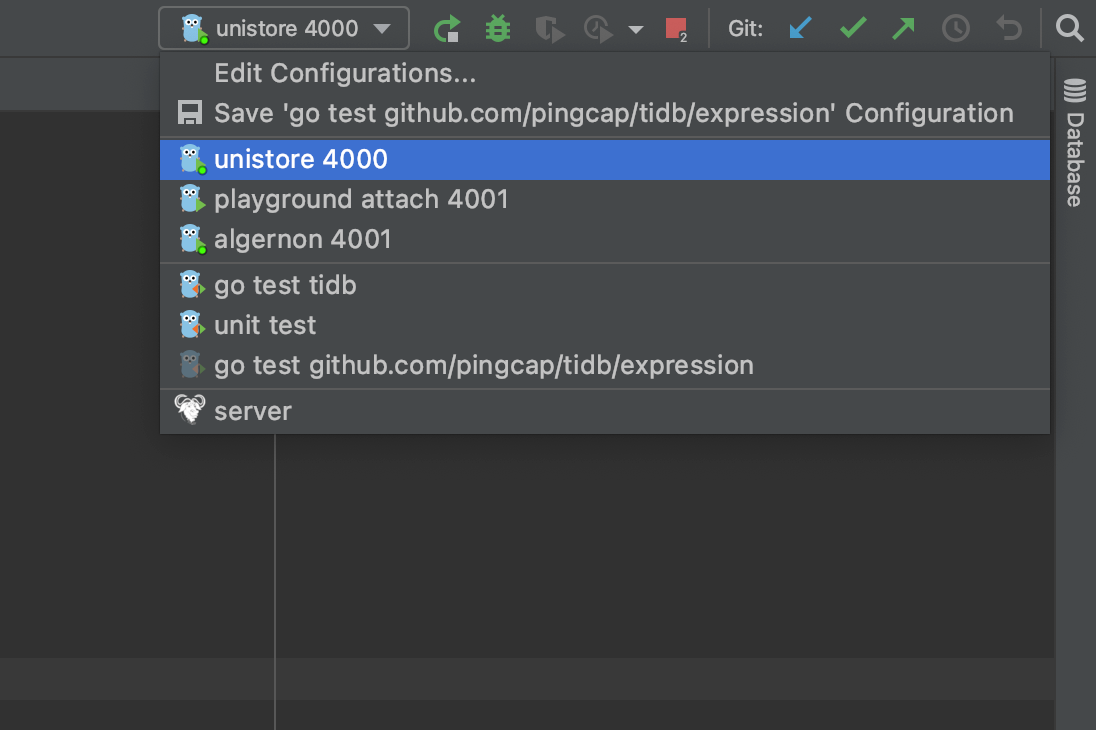
The first config is unistore 4000, which enables you to run/debug TiDB independently without TiKV, PD, and TiFlash.
The second config is playground attach 4001, which enables you to run/debug TiDB by attaching to an existing cluster; for example, a cluster deployed with tiup playground.
After the server process starts, you can connect to the origin TiDB by port 4000, or connect to your TiDB by port 4001 at the same time.
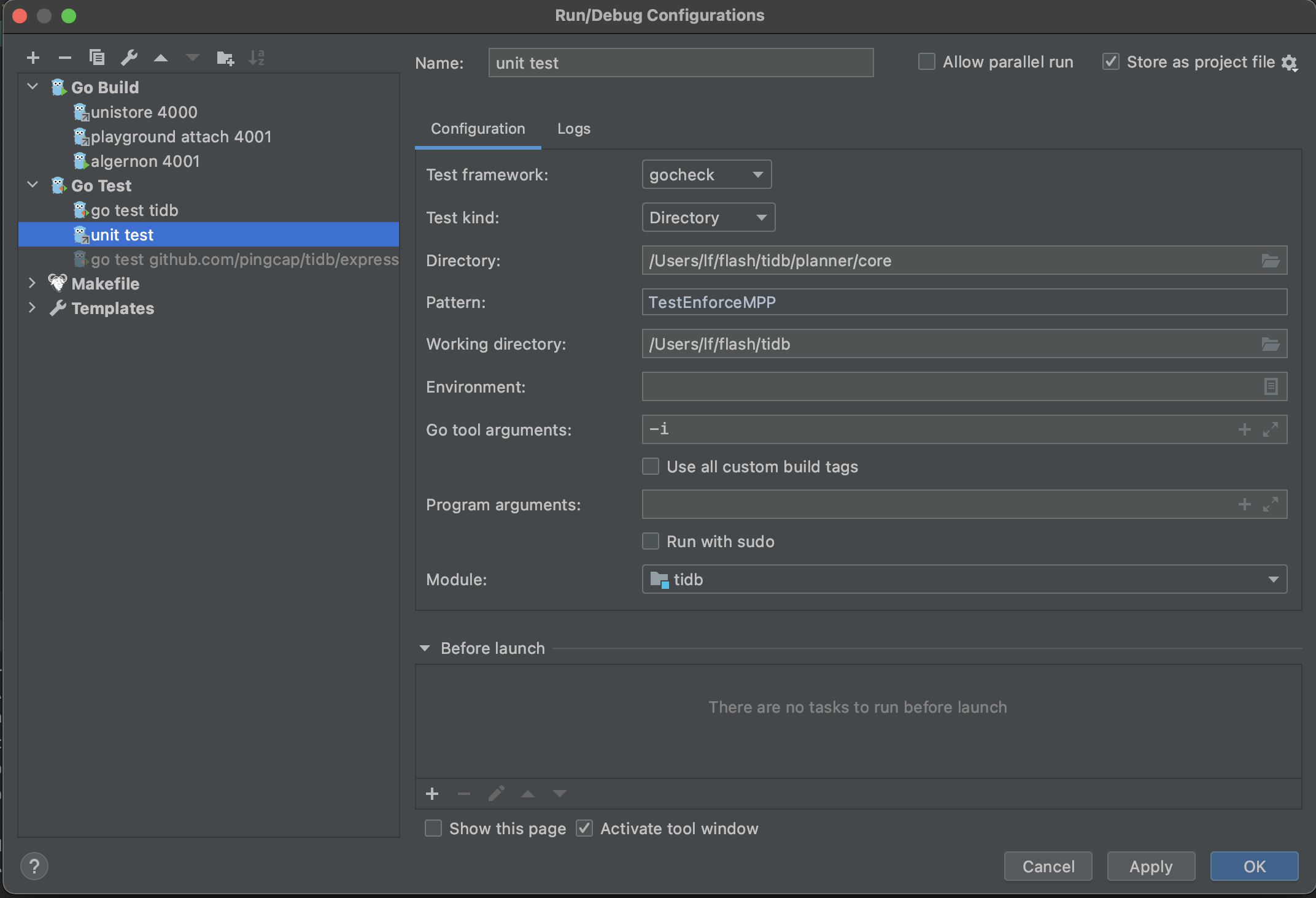
The third config is unit test, which enables you to run/debug unit tests. You may modify the Directory and Pattern to run other tests.
If you encounter any problems during your journey, do not hesitate to reach out on the TiDB Internals forum.
Visual Studio Code
VS Code is a generic IDE that has good extensions for working with Go and TiDB.
Prerequisites
go: TiDB is a Go project thus its building requires a workinggoenvironment. See the previous Install Golang section to prepare the environment.- TiDB source code: See the previous Get the code, build and run section to get the source code.
Download VS Code
Download VS Code from here and install it.
Now install these extensions:
Work with TiDB code in VS Code
Open the folder containing TiDB code via File→Open Folder. See the VS Code docs for how to edit and commit code.
There is detailed guide explaining how to use the TiDE extension.
Populate run configurations
Under the root directory of the TiDB source code, execute the following commands to add config files:
mkdir -p .vscode

echo "{
    \"go.testTags\": \"intest,deadlock\"
}" > .vscode/settings.json
Write and run unit tests
The Golang testing framework provides several functionalities and conventions that help structure and execute tests efficiently. To enhance its assertion and mocking capabilities, we use the testify library.
You may find tests using pingcap/check which is a fork of go-check/check in release branches before
release-6.1, but since that framework is poorly maintained, we are migrated to testify fromrelease-6.1. You can check the background and progress on the migration tracking issue.
How to write unit tests
We use testify to write unit tests. Basically, it is out-of-the-box testing with testify assertions.
TestMain
When you run tests, Golang compiles each package along with any files with names with suffix _test.go. Thus, a test binary contains tests in a package.
Golang testing provides a mechanism to support doing extra setup or teardown before or after testing by writing a package level unique function:
func TestMain(m *testing.M)
After all tests finish, we leverage the function to detect Goroutine leaks by goleak.
Before you write any unit tests in a package, create a file named main_test.go and setup the scaffolding:
func TestMain(m *testing.M) {
    goleak.VerifyTestMain(m)
}
You can also put global variables or helper functions of the test binary in this file.
Assertion
Let's write a basic test for the utility function StrLenOfUint64Fast:
func TestStrLenOfUint64Fast(t *testing.T) {
    for i := 0; i < 1000000; i++ {
        num := rand.Uint64()
        expected := len(strconv.FormatUint(num, 10))
        actual := StrLenOfUint64Fast(num)
        require.Equal(t, expected, actual)
    }
}
Golang testing detects test functions from *_test.go files of the form:
func TestXxx(*testing.T)
where Xxx does not start with a lowercase letter. The function name identifies the test routine.
We follow this pattern but use testify assertions instead of out-of-the-box methods, like Error or Fail, since they are too low level to use.
We mostly use require.Xxx for assertions, which is imported from github.com/stretchr/testify/require. If the assertions fail, the test fails immediately, and we tend to fail tests fast.
Below are the most frequently used assertions:
func Equal(t TestingT, expected interface{}, actual interface{}, msgAndArgs ...interface{})
func EqualValues(t TestingT, expected interface{}, actual interface{}, msgAndArgs ...interface{})
func Len(t TestingT, object interface{}, length int, msgAndArgs ...interface{})
func Nil(t TestingT, object interface{}, msgAndArgs ...interface{})
func NoError(t TestingT, err error, msgAndArgs ...interface{})
func NotNil(t TestingT, object interface{}, msgAndArgs ...interface{})
func True(t TestingT, value bool, msgAndArgs ...interface{})
You can find other assertions follow the documentation.
Parallel
Golang testing provides a method of testing.T to run tests in parallel:
t.Parallel()
We leverage this function to run tests as parallel as possible, so that we make full use of the available resource.
When some tests should be run in serial, use Golang testing subtests and parallel the parent test only. In this way, tests in the same subtests set run in serial.
func TestParent(t *testing.T) {
    t.Parallel()
    // <setup code>
    t.Run("Serial 0", func(t *testing.T) { ... })
    t.Run("Serial 1", func(t *testing.T) { ... })
    t.Run("Serial 2", func(t *testing.T) { ... })
    // <tear-down code>
}
Generally, if a test modifies global configs or fail points, it should be run in serial.
When writing parallel tests, there are several common considerations.
In Golang, the loop iterator variable is a single variable that takes different value in each loop iteration. Thus, when you run this code it is highly possible to see the last element used for every iteration. You may use below paradigm to work around.
func TestParallelWithRange(t *testing.T) {
    for _, test := range tests {
        // copy iterator variable into a new variable, see issue #27779 in tidb repo
        test := test
        t.Run(test.Name, func(t *testing.T) {
            t.Parallel()
            ...
        })
    }
}
Test kits
Most of our tests are much more complex than what we describe above. For example, to set up a test, we may create a mock storage, a mock session, or even a local database instance.
These functions are known as test kits. Some are used in one package so we implement them in place; others are quite common so we move it to the testkit directory.
When you write complex unit tests, you may take a look at what test kits we have now and try to leverage them. If we don’t have a test kit for your issue and your issue is considered common, add one.
How to run unit tests
Running all tests
You can always run all tests by executing the ut (stands for unit test) target in Makefile:
make ut
This is almost equivalent to go test ./... but it enables and disables fail points before and after running tests.
pingcap/failpoint is an implementation of failpoints for Golang. A fail point is used to add code points where you can inject errors. Fail point is a code snippet that is only executed when the corresponding fail point is active.
Running a single test
To run a single test, you can manually repeat what make ut does and narrow the scope in one test or one package:
make failpoint-enable
cd pkg/domain
go test -v -run TestSchemaValidator # or with any other test flags
cd ../..
make failpoint-disable
or if it is an older test not using testify
make failpoint-enable
(cd pkg/planner/core ; go test -v -run "^TestT$" -check.f TestBinaryOpFunction )
make failpoint-disable
If one want to compile the test into a debug binary for running in a debugger, one can also use go test -gcflags="all=-N -l" -o ./t, which removes any optimisations and outputs a t binary file ready to be used, like dlv exec ./t or combine it with the above to only debug a single test dlv exec ./t -- -test.run "^TestT$" -check.f TestBinaryOpFunction.
Notice there is also an ut utility for running tests, see Makefile and tools/bin/ut.
To display information on all the test flags, enter go help testflag.
If you develop with GoLand, you can also run a test from the IDE with manually enabled and disabled fail points. See the documentation for details.
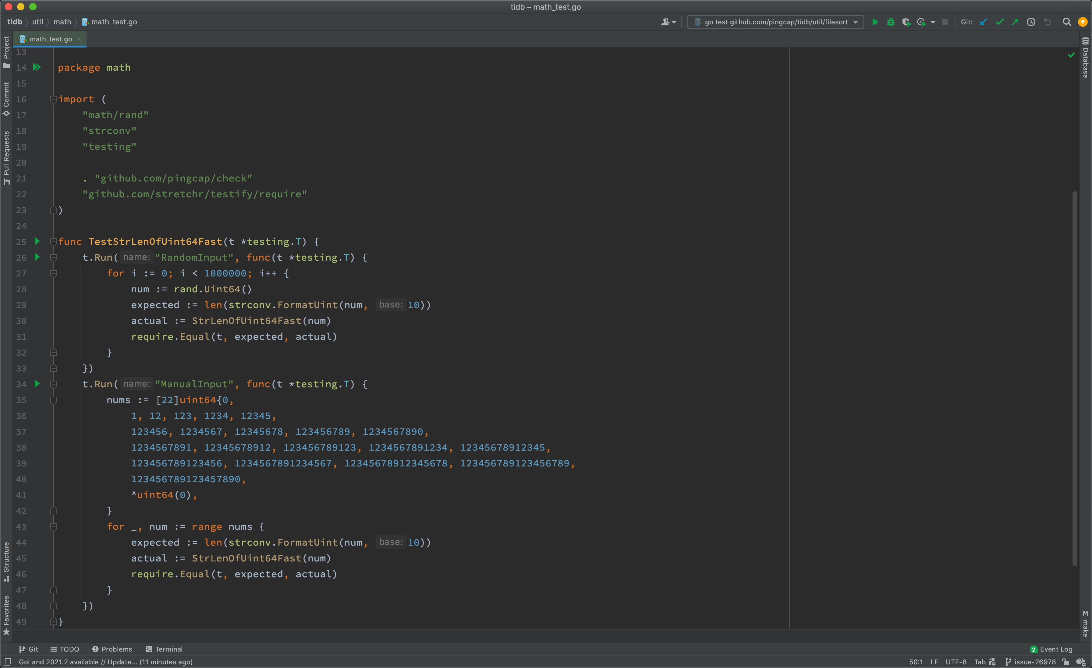
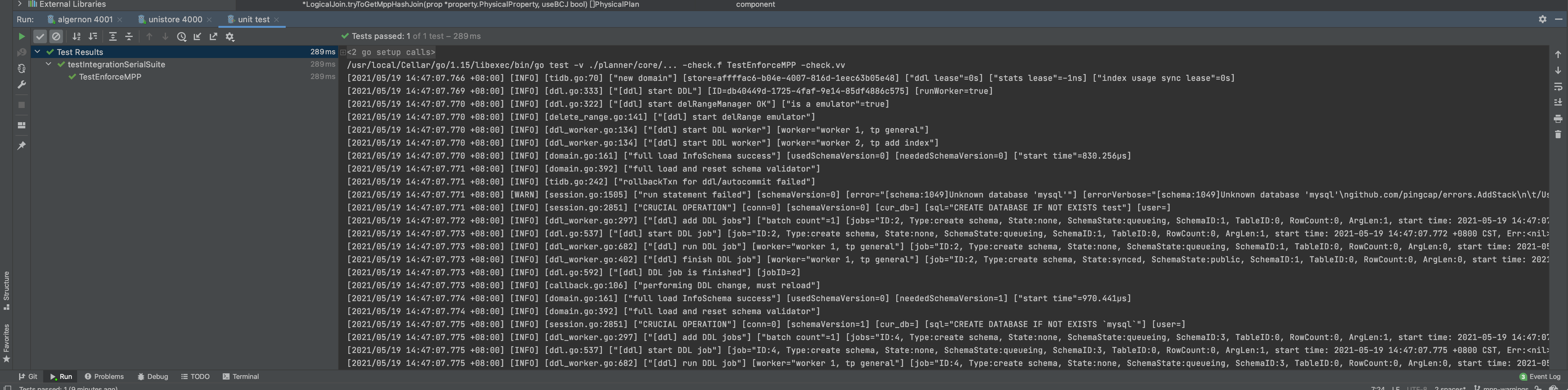
As shown above, you can run tests of the whole package, of a test, or of a subtest, by click the corresponding gutter icon.
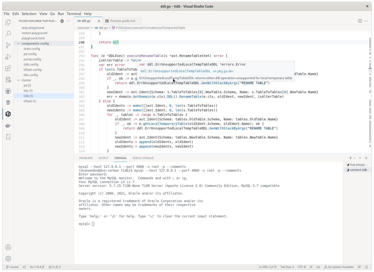
If you develop with VS Code, you can also run a test from the editor with manually enabled and disabled fail points. See the documentation for details.
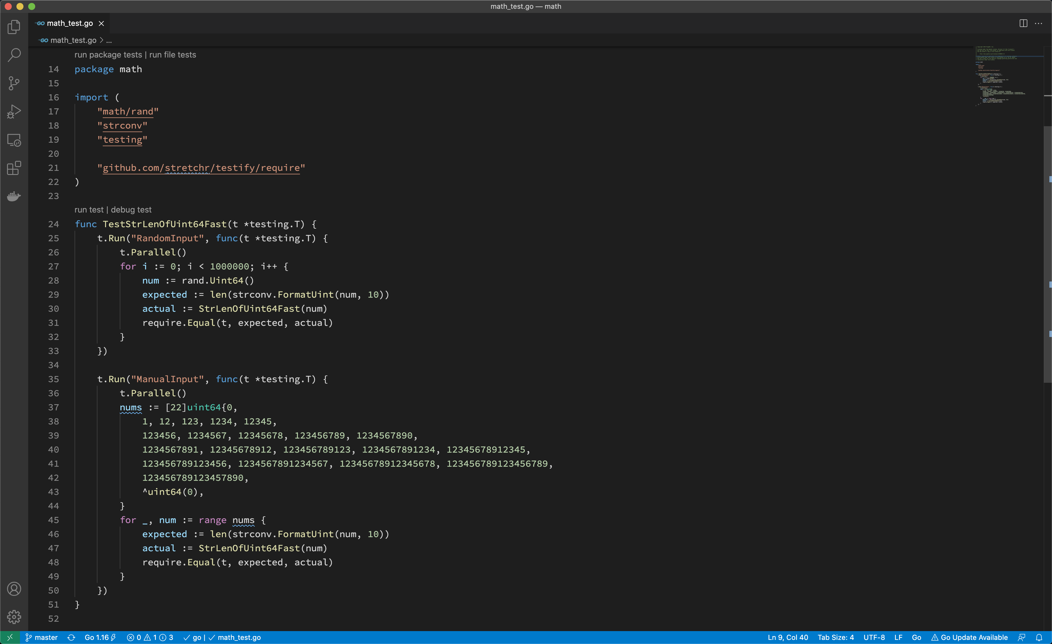
As shown above, you can run tests of the whole package, of a test, or of a file.
Running tests for a pull request
If you haven't joined the organization, you should wait for a member to comment with
/ok-to-testto your pull request.
Before you merge a pull request, it must pass all tests.
Generally, continuous integration (CI) runs the tests for you; however, if you want to run tests with conditions or rerun tests on failure, you should know how to do that, the rerun guide comment will be sent when the CI tests failed.
/retest
Rerun all failed CI test cases.
/test {{test1}} {{testN}}
Run given CI failed tests.
CI parameters
CI jobs accepts the following parameters passed from pull request title:
format: <origin pr title> | <the CI args pairs>
CI args pairs:
tikv=<branch>|<pr/$num>specifies which tikv to use.pd=<branch>|<pr/$num>specifies which pd to use.tidb-test=<branch>|<pr/$num>specifies which tidb-test to use.
For example:
pkg1: support xxx feature | tidb-test=pr/1234
pkg2: support yyy feature | tidb-test=release-6.5 tikv=pr/999
How to find failed tests
There are several common causes of failed tests.
Assertion failed
The most common cause of failed tests is that assertion failed. Its failure report looks like:
=== RUN   TestTopology
    info_test.go:72:
            Error Trace:    info_test.go:72
            Error:          Not equal:
                            expected: 1282967700000
                            actual  : 1628585893
            Test:           TestTopology
--- FAIL: TestTopology (0.76s)
To find this type of failure, enter grep -i "FAIL" to search the report output.
Data race
Golang testing supports detecting data race by running tests with the -race flag. Its failure report looks like:
[2021-06-21T15:36:38.766Z] ==================
[2021-06-21T15:36:38.766Z] WARNING: DATA RACE
[2021-06-21T15:36:38.766Z] Read at 0x00c0055ce380 by goroutine 108:
...
[2021-06-21T15:36:38.766Z] Previous write at 0x00c0055ce380 by goroutine 169:
[2021-06-21T15:36:38.766Z]   [failed to restore the stack]
Goroutine leak
We use goleak to detect goroutine leak for tests. Its failure report looks like:
goleak: Errors on successful test run: found unexpected goroutines:
[Goroutine 104 in state chan receive, with go.etcd.io/etcd/pkg/logutil.(*MergeLogger).outputLoop on top of the stack:
goroutine 104 [chan receive]:
go.etcd.io/etcd/pkg/logutil.(*MergeLogger).outputLoop(0xc000197398)
    /go/pkg/mod/go.etcd.io/etcd@v0.5.0-alpha.5.0.20200824191128-ae9734ed278b/pkg/logutil/merge_logger.go:173 +0x3ac
created by go.etcd.io/etcd/pkg/logutil.NewMergeLogger
    /go/pkg/mod/go.etcd.io/etcd@v0.5.0-alpha.5.0.20200824191128-ae9734ed278b/pkg/logutil/merge_logger.go:91 +0x85
To determine the source of package leaks, see the documentation
Timeout
After @tiancaiamao introduced the timeout checker for continuous integration, every test case should run in at most five seconds.
If a test case takes longer, its failure report looks like:
[2021-08-09T03:33:57.661Z] The following test cases take too long to finish:
[2021-08-09T03:33:57.661Z] PASS: tidb_test.go:874: tidbTestSerialSuite.TestTLS  7.388s
[2021-08-09T03:33:57.661Z] --- PASS: TestCluster (5.20s)
And for integration tests, please refer to Run and debug integration tests
Debug and profile
In this section, you will learn:
- How to debug TiDB
- How to pause the execution at any line of code to inspect values and stacks
- How to profile TiDB to catch a performance bottleneck
Use delve for debugging
Delve is a debugger for the Go programming language. It provides a command-line debugging experience similar to the GNU Project debugger (GDB), but it is much more Go native than GDB itself.
Install delve
To install delve, see the installation guide. After the installation, depending on how you set your environment variables, you will have an executable file named dlv in either $GOPATH/bin or $HOME/go/bin. You can then run the following command to verify the installation:
$ dlv version
Delve Debugger
Version: 1.5.0
Build: $Id: ca5318932770ca063fc9885b4764c30bfaf8a199 $
Attach delve to a running TiDB process
Once you get the TiDB server running, you can attach the delve debugger.
For example, you can build and run a standalone TiDB server by running the following commands in the root directory of the source code:
make server
./bin/tidb-server
You can then start a new shell and use ps or pgrep to find the PID of the tidb server process you just started:
pgrep tidb-server
# OUTPUT:
# 1394942
If the output lists multiple PIDs, it indicates that you might have multiple TiDB servers running at the same time. To determine the PID of the tidb server you are planning to debug, you can use commands such as ps $PID, where $PID is the PID you are trying to know more about:
ps 1394942
# OUTPUT:
#     PID TTY      STAT   TIME COMMAND
# 1394942 pts/11   SNl    0:02 ./bin/tidb-server
Once you get the PID, you can attach delve to it by running the following command:
dlv attach 1394942
You might get error messages of the kernel security setting as follows:
Could not attach to pid 1394942: this could be caused by a kernel security setting, try writing "0" to /proc/sys/kernel/yama/ptrace_scope
To resolve the error, follow the instructions provided in the error message and execute the following command as the root user to override the kernel security setting:
echo 0 > /proc/sys/kernel/yama/ptrace_scope
Then retry attaching delve onto the PID, and it should work.
If you've worked with GDB, the delve debugging interface will look familiar to you. It is an interactive dialogue that allows you to interact with the execution of the tidb server attached on. To learn more about delve, you can type help into the dialogue and read the help messages.
Use delve for debugging
After attaching delve to the running TiDB server process, you can now set breakpoints. TiDB server will pause execution at the breakpoints you specify.
To create a breakpoint, you can write:
break [name] <linespec>
where [name] is the name for the breakpoint, and <linespec> is the position of a line of code in the source code. Note the name is optional.
For example, the following command creates a breakpoint at the Next function of HashJoinExec. (The line number can be subject to change due to the modification of the source code).
dlv debug tidb-server/main.go
# OUTPUT:
# Type 'help' for list of commands.
# (dlv) break executor/join.go:653
# Breakpoint 1 (enabled) set at 0x36752d8 for github.com/pingcap/tidb/executor.(*HashJoinExec).Next() ./executor/join.go:653
# (dlv)
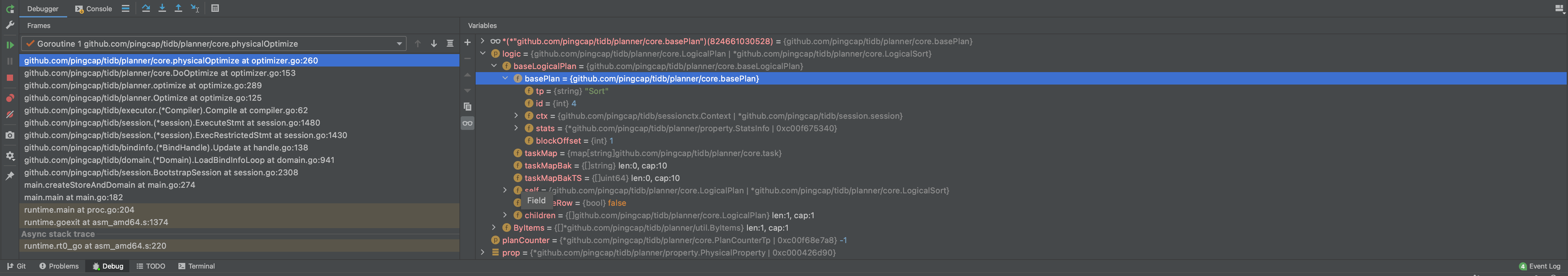
Once the execution is paused, the context of the execution is fully preserved. You are free to inspect the values of different variables, print the calling stack, and even jump between different goroutines. Once you finish the inspection, you can resume the execution by stepping into the next line of code or continue the execution until the next breakpoint is encountered.
Typically, when you use a debugger, you need to take the following steps:
- Locate the code and set a breakpoint.
- Prepare data so that the execution will get through the breakpoint, and pause at the specified breakpoint as expected.
- Inspect values and follow the execution step by step.
Using delve to debug a test case
If a test case fails, you can also use delve to debug it. Get the name of the test case, go to the corresponding package directory, and then run the following command to start a debugging session that will stop at the entry of the test:
dlv test -- -run TestName
Understand how TiDB works through debugging
Besides debugging problems, you can also use the debugger to understand how TiDB works through tracking the execution step by step.
To understand TiDB internals, it's critical that you understand certain functions. To better understand how TiDB works, you can pause the execution of these TiDB functions, and then run TiDB step by step.
For example:
executor/compiler.go:Compileis where each SQL statement is compiled and optimized.planner/planner.go:Optimizeis where the SQL optimization starts.executor/adapter.go:ExecStmt.Execis where the SQL plan turns into executor and where the SQL execution starts.- Each executor's
Open,Next, andClosefunction marks the volcano-style execution logic.
When you are reading the TiDB source code, you are strongly encouraged to set a breakpoint and use the debugger to trace the execution whenever you are confused or uncertain about the code.
Using pprof for profiling
For any database system, performance is always important. If you want to know where the performance bottleneck is, you can use a powerful Go profiling tool called pprof.
Gather runtime profiling information through HTTP end points
Usually, when TiDB server is running, it exposes a profiling end point through HTTP at http://127.0.0.1:10080/debug/pprof/profile. You can get the profile result by running the following commands:
curl -G "127.0.0.1:10080/debug/pprof/profile?seconds=45" > profile.profile
go tool pprof -http 127.0.0.1:4001 profile.profile
The commands capture the profiling information for 45 seconds, and then provide a web view of the profiling result at 127.0.0.1:4001. This view contains a flame graph of the execution and more views that can help you diagnose the performance bottleneck.
You can also gather other runtime information through this end point. For example:
- Goroutine:
curl -G "127.0.0.1:10080/debug/pprof/goroutine" > goroutine.profile
- Trace:
curl -G "127.0.0.1:10080/debug/pprof/trace?seconds=3" > trace.profile
go tool trace -http 127.0.0.1:4001 trace.profile
- Heap:
curl -G "127.0.0.1:10080/debug/pprof/heap" > heap.profile
go tool pprof -http 127.0.0.1:4001 heap.profile
To learn how the runtime information is analyzed, see Go's diagnostics document.
Profiling during benchmarking
When you are proposing a performance-related feature for TiDB, we recommend that you also include a benchmark result as proof of the performance gain or to show that your code won't introduce any performance regression. In this case, you need to write your own benchmark test like in executor/benchmark.go.
For example, if you want to benchmark the window functions, because BenchmarkWindow are already in the benchmark tests, you can run the following commands to get the benchmark result:
cd executor
go test -bench BenchmarkWindow -run BenchmarkWindow -benchmem
If you find any performance regression, and you want to know the cause of it, you could use a command like the following:
go test -bench BenchmarkWindow -run BenchmarkWindow -benchmem -memprofile memprofile.out -cpuprofile profile.out
Then, you can use the steps described above to generate and analyze the profiling information.
Commit the code and submit a pull request
The TiDB project uses Git to manage its source code. To contribute to the project, you need to get familiar with Git features so that your changes can be incorporated into the codebase.
This section addresses some of the most common questions and problems that new contributors might face. This section also covers some Git basics; however if you find that the content is a little difficult to understand, we recommend that you first read the following introductions to Git:
- The "Beginner" and "Getting Started" sections of this tutorial from Atlassian
- Documentation and guides for beginners from Github
- A more in-depth book from Git
Prerequisites
Before you create a pull request, make sure that you've installed Git, forked pingcap/tidb, and cloned the upstream repo to your PC. The following instructions use the command line interface to interact with Git; there are also several GUIs and IDE integrations that can interact with Git too.
If you've cloned the upstream repo, you can reference it using origin in your local repo. Next, you need to set up a remote for the repo your forked using the following command:
git remote add dev https://github.com/your_github_id/tidb.git
You can check the remote setting using the following command:
git remote -v
# dev    https://github.com/username/tidb.git (fetch)
# dev    https://github.com/username/tidb.git (push)
# origin    https://github.com/pingcap/tidb.git (fetch)
# origin    https://github.com/pingcap/tidb.git (push)
Standard Process
The following is a normal procedure that you're likely to use for the most common minor changes and PRs:
-
Ensure that you're making your changes on top of master and get the latest changes:
git checkout master git pull master -
Create a new branch for your changes:
git checkout -b my-changes -
Make some changes to the repo and test them.
If the repo is buiding with Bazel tool, you should update the bazel files(*.bazel, DEPS.bzl) also.
-
Commit your changes and push them to your
devremote repository:# stage files you created/changed/deleted git add path/to/changed/file.go path/to/another/changed/file.go # commit changes staged, make sure the commit message is meaningful and readable git commit -s -m "pkg, pkg2, pkg3: what's changed" # optionally use `git status` to check if the change set is correct # git status # push the change to your `dev` remote repository git push --set-upstream dev my-changes -
Make a PR from your fork to the master branch of pingcap/tidb. For more information on how to make a PR, see Making a Pull Request in GitHub Guides.
When making a PR, look at the PR template and follow the commit message format, PR title format, and checklists.
After you create a PR, if your reviewer requests code changes, the procedure for making those changes is similar to that of making a PR, with some steps skipped:
-
Switch to the branch that is the head and get the latest changes:
git checkout my-changes git pull -
Make, stage, and commit your additional changes just like before.
-
Push those changes to your fork:
git push
If your reviewer requests for changes with GitHub suggestion, you can commit the suggestion from the webpage. GitHub provides documentation for this case.
Conflicts
When you edit your code locally, you are making changes to the version of pingcap/tidb that existed when you created your feature branch. As such, when you submit your PR it is possible that some of the changes that have been made to pingcap/tidb since then conflict with the changes you've made.
When this happens, you need to resolve the conflicts before your changes can be merged. First, get a local copy of the conflicting changes: checkout your local master branch with git checkout master, then git pull master to update it with the most recent changes.
Rebasing
You're now ready to start the rebasing process. Checkout the branch with your changes and execute git rebase master.
When you rebase a branch on master, all the changes on your branch are reapplied to the most recent version of master. In other words, Git tries to pretend that the changes you made to the old version of master were instead made to the new version of master. During this process, you should expect to encounter at least one "rebase conflict." This happens when Git's attempt to reapply the changes fails because your changes conflict with other changes that have been made. You can tell that this happened because you'll see lines in the output that look like:
CONFLICT (content): Merge conflict in file.go
When you open these files, you'll see sections of the form
<<<<<<< HEAD
Original code
=======
Your code
>>>>>>> 8fbf656... Commit fixes 12345
This represents the lines in the file that Git could not figure out how to rebase. The section between <<<<<<< HEAD and ======= has the code from master, while the other side has your version of the code. You'll need to decide how to deal with the conflict. You may want to keep your changes, keep the changes on master, or combine the two.
Generally, resolving the conflict consists of two steps: First, fix the particular conflict. Edit the file to make the changes you want and remove the <<<<<<<, =======, and >>>>>>> lines in the process. Second, check the surrounding code. If there was a conflict, it's likely there are some logical errors lying around too!
Once you're all done fixing the conflicts, you need to stage the files that had conflicts in them via git add. Afterwards, run git rebase --continue to let Git know that you've resolved the conflicts and it should finish the rebase.
Once the rebase has succeeded, you'll want to update the associated branch on your fork with git push --force-with-lease.
Advanced rebasing
If your branch contains multiple consecutive rewrites of the same code, or if the rebase conflicts are extremely severe, you can use git rebase --interactive master to gain more control over the process. This allows you to choose to skip commits, edit the commits that you do not skip, change the order in which they are applied, or "squash" them into each other.
Alternatively, you can sacrifice the commit history like this:
# squash all the changes into one commit so you only have to worry about conflicts once
git rebase -i $(git merge-base master HEAD)  # and squash all changes along the way
git rebase master
# fix all merge conflicts
git rebase --continue
Squashing commits into each other causes them to be merged into a single commit. Both the upside and downside of this is that it simplifies the history. On the one hand, you lose track of the steps in which changes were made, but the history becomes easier to work with.
You also may want to squash together just the last few commits, possibly because they only represent "fixups" and not real changes. For example, git rebase --interactive HEAD~2 allows you to edit the two commits only.
Setting pre-commit
We use pre-commit to check the code style before committing. To install pre-commit, run:
# Using pip:
pip install pre-commit

# Using homebrew:
brew install pre-commit
After the installation is successful, run pre-commit install in the project root directory to enable git's pre-commit.
Contribute to TiDB
TiDB is developed by an open and friendly community. Everybody is cordially welcome to join the community and contribute to TiDB. We value all forms of contributions, including, but not limited to:
- Code reviewing of the existing patches
- Documentation and usage examples
- Community participation in forums and issues
- Code readability and developer guide
- We welcome contributions that add code comments and code refactor to improve readability
- We also welcome contributions to docs to explain the design choices of the internal
- Test cases to make the codebase more robust
- Tutorials, blog posts, talks that promote the project
Here are guidelines for contributing to various aspect of the project:
- Community Guideline
- Report an Issue
- Issue Triage
- Contribute Code
- Cherry-pick a Pull Request
- Review a Pull Request
- Make a Proposal
- Code Style and Quality Guide
- Write Document
- Release Notes Language Style Guide
- Committer Guide
- Miscellaneous Topics
Any other question? Reach out to the TiDB Internals forum to get help!
Community Guideline
TiDB community aims to provide harassment-free, welcome and friendly experience for everyone. The first and most important thing for any participant in the community is be friendly and respectful to others. Improper behaviors will be warned and punished.
We appreciate any contribution in any form to TiDB community. Thanks so much for your interest and enthusiasm on TiDB!
Code of Conduct
TiDB community refuses any kind of harmful behavior to the community or community members. Everyone should read our Code of Conduct and keep proper behavior while participating in the community.
Governance
TiDB development governs by two kind of groups:
- TOC: TOC serves as the main bridge and channel for coordinating and information sharing across companies and organizations. It is the coordination center for solving problems in terms of resource mobilization, technical research and development direction in the current community and cooperative projects.
- teams: Teams are persistent open groups that focus on a part of the TiDB projects. A team has its reviewer, committer and maintainer, and owns one or more repositories. Team level decision making comes from its maintainers.
A typical promoted path for a TiDB developer is from user to reviewer, then committer and maintainer, finally maybe a TOC member. But gaining more roles doesn't mean you have any privilege over other community members or even any right to control them. Everyone in TiDB community are equal and share the responsibility to collaborate constructively with other contributors, building a friendly community. The roles are a natural reward for your substantial contribution in TiDB development and provide you more rights in the development workflow to enhance your efficiency. Meanwhile, they request some additional responsibilities from you:
- Now that you are a member of team reviewers/committers/maintainers, you are representing the project and your fellow team members whenever you discuss TiDB with anyone. So please be a good person to defend the reputation of the team.
- Committers/maintainers have the right to approve pull requests, so bear the additional responsibility of handling the consequences of accepting a change into the codebase or documentation. That includes reverting or fixing it if it causes problems as well as helping out the release manager in resolving any problems found during the pre-release testing cycle. While all contributors are free to help out with this part of the process, and it is most welcome when they do, the actual responsibility rests with the committers/maintainers that approved the change.
- Reviewers/committers/maintainers also bear the primary responsibility for guiding contributors the right working procedure, like deciding when changes proposed on the issue tracker should be escalated to internal.tidb.io for wider discussion, as well as suggesting the use of the TiDB Design Documents process to manage the design and justification of complex changes, or changes with a potentially significant impact on end users.
There should be no blockers to contribute with no roles. It's totally fine for you to reject the promotion offer if you don't want to take the additional responsibilities or for any other reason. Besides, except for code or documentation contribution, any kind of contribution for the community is highly appreciated. Let's grow TiDB ecosystem through our contributions of this community.
Report an Issue
If you think you have found an issue in TiDB, you can report it to the issue tracker. If you would like to report issues to TiDB documents or this development guide, they are in separate GitHub repositories, so you need to file issues to corresponding issue tracker, TiDB document issue tracker and TiDB Development Guide issue tracker. Read Write Document for more details.
Checking if an issue already exists
The first step before filing an issue report is to see whether the problem has already been reported. You can use the search bar to search existing issues. This doesn't always work, and sometimes it's hard to know what to search for, so consider this extra credit. We won't mind if you accidentally file a duplicate report. Don't blame yourself if your issue is closed as duplicated. We highly recommend if you are not sure about anything of your issue report, you can turn to internal.tidb.io for a wider audience and ask for discussion or help.
Filing an issue
If the problem you're reporting is not already in the issue tracker, you can open a GitHub issue with your GitHub account. TiDB uses issue template for different kinds of issues. Issue templates are a bundle of questions to collect necessary information about the problem to make it easy for other contributors to participate. For example, a bug report issue template consists of four questions:
- Minimal reproduce step.
- What did you expect to see?
- What did you see instead?
- What is your TiDB version?
Answering these questions give the details about your problem so other contributors or TiDB users could pick up your issue more easily.
As previous section shows, duplicated issues should be reduced. To help others who encountered the problem find your issue, except for problem details answered in the issue template, a descriptive title which contains information that might be unique to it also helps. This can be the components your issue belongs to or database features used in your issue, the conditions that trigger the bug, or part of the error message if there is any.
Making good issues
Except for a good title and detailed issue message, you can also add suitable labels to your issue via /label, especially which component the issue belongs to and which versions the issue affects. Many committers and contributors only focus on certain subsystems of TiDB. Setting the appropriate component is important for getting their attention. Some issues might affect multiple releases. You can query Issue Triage chapter for more information about what need to do with such issues.
If you are able to, you should take more considerations on your issue:
- Does the feature fit well into TiDB's architecture? Will it scale and keep TiDB flexible for the future, or will the feature restrict TiDB in the future?
- Is the feature a significant new addition (rather than an improvement to an existing part)? If yes, will the community commit to maintaining this feature?
- Does this feature align well with currently ongoing efforts?
- Does the feature produce additional value for TiDB users or developers? Or does it introduce the risk of regression without adding relevant user or developer benefit?
Deep thoughts could help the issue proceed faster and help build your own reputation in the community.
Understanding the issue's progress and status
Once your issue is created, other contributors might take part in. You need to discuss with them, provide more information they might want to know, address their comments to reach consensus and make the progress proceeds. But please realize there are always more pending issues than contributors are able to handle, and especially TiDB community is a global one, contributors reside all over the world and they might already be very busy with their own work and life. Please be patient! If your issue gets stale for some time, it's okay to ping other participants, or take it to internal.tidb.io for more attention.
Disagreement with a resolution on the issue tracker
As humans, we will have differences of opinions from time to time. First and foremost, please be respectful that care, thought, and volunteer time went into the resolution.
With this in mind, take some time to consider any comments made in association with the resolution of the issue. On reflection, the resolution steps may seem more reasonable than you initially thought.
If you still feel the resolution is incorrect, then raise a thoughtful question on internal.tidb.io. Further argument and disrespectful discourse on internal.tidb.io after a consensus has been reached amongst the committers is unlikely to win any converts.
Reporting security vulnerabilities
Security issues are not suitable to report in public early, so different tracker strategy is used. Please refer to the dedicated process.
Issue Triage
TiDB uses an issue-centric workflow for development. Every problem, enhancement and feature starts with an issue. For bug issues, you need to perform some more triage operations on the issues.
Diagnose issue severity
The severity of a bug reflects the level of impact that the bug has on users when they use TiDB. The greater the impact, the higher severity the bug is. For higher severity bugs, we need to fix them faster. Although the impact of bugs can not be exhausted, they can be divided into four levels.
Critical
The bug affects critical functionality or critical data. It might cause huge losses to users and does not have a workaround. Some typical critical bugs are as follows:
- Invalid query result (correctness issues)
- TiDB returns incorrect results or results that are in the wrong order for a typical user-written query.
- Bugs caused by type casts.
- The parameters are not boundary value or invalid value, but the query result is not correct(except for overflow scenes).
- Incorrect DDL and DML result
- The data is not written to the disk, or wrong data is written.
- Data and index are inconsistent.
- Invalid features
- Due to a regression, the feature can not work in its main workflow
- Follower can not read follower.
- SQL hint does not work.
- SQL Plan
- Cannot choose the best index. The difference between best plan and chosen plan is bigger than 200%.
- DDL design
- DDL process causes data accuracy issue.
- Experimental feature
- If the issue leads to another stable feature’s main workflow not work, and may occur on released version, the severity is critical.
- If the issue leads to data loss, the severity is critical.
- Exceptions
- If the feature is clearly labeled as experimental, when it doesn’t work but doesn’t impact another stable feature’s main workflow or only impacts stable feature’s main workflow on master, the issue severity is major.
- The feature has been deprecated and a viable workaround is available(at most major).
- Due to a regression, the feature can not work in its main workflow
- System stability
- The system is unavailable for more than 5 minutes(if there are some system errors, the timing starts from failure recovery).
- Tools cannot perform replication between upstream and downstream for more than 1 minute if there are no system errors.
- TiDB cannot perform the upgrade operation.
- TPS/QPS dropped 25% without system errors or rolling upgrades.
- Unexpected TiKV core dump or TiDB panic(process crashed).
- System resource leak, include but not limit to memory leak and goroutine leak.
- System fails to recover from crash.
- Security and compliance issues
- CVSS score >= 9.0.
- TiDB leaks secure information to log files, or prints customer data when set to be desensitized.
- Backup or Recovery Issues
- Failure to either backup or restore is always considered critical.
- Incompatible Issues
- Syntax/compatibility issue affecting default install of tier 1 application(i.e. Wordpress).
- The DML result is incompatible with MySQL.
- CI test case fail
- Test cases which lead to CI failure and could always be reproduced.
- Bug location information
- Key information is missing in ERROR level log.
- No data is reported in monitor.
Major
The bug affects major functionality. Some typical critical bugs are as follow:
- Invalid query result
- The query gets the wrong result caused by overflow.
- The query gets the wrong result in the corner case.
- For boundary value, the processing logic in TiDB is inconsistent with MySQL.
- Inconsistent data precision.
- Incorrect DML or DDL result
- Extra or wrong data is written to TiDB with a DML in a corner case.
- Invalid features
- The corner case of the main workflow of the feature does not work.
- The feature is experimental, but a main workflow does not work.
- Incompatible issue of view functionality.
- SQL Plan
- Choose sub-optimal plan. The difference between best plan and chosen plan is bigger than 100% and less than 200%
- System stability
- TiDB panics but process does not exit.
- Less important security and compliance issues
- CVSS score >= 7.0
- Issues that affects critical functionality or critical data but rare to reproduce(can’t be reproduced in one week, and have no clear reproduce steps)
- CI test cases fail
- Test case is not stable.
- Bug location information
- Key information is missing in WARN level log.
- Data is not accurate in monitor.
Moderate
- SQL Plan
- Cannot get the best plan due to invalid statistics.
- Documentation issues
- The bugs were caused by invalid parameters which rarely occurred in the product environment.
- Security issues
- CVSS score >= 4.0
- Incompatible issues occurred on boundary value
- Bug location information
- Key information is missing in DEBUG/INFO level log.
Minor
The bug does not affect functionality or data. It does not even need a workaround. It does not impact productivity or efficiency. It is merely an inconvenience. For example:
- Invalid notification
- Minor compatibility issues
- Error message or error code does not match MySQL.
- Issues caused by invalid parameters or abnormal cases.
Not a bug
The following issues look like bugs but actually not. They should not be labeled type/bug and instead be only labeled type/compatibility:
- Behavior is different from MySQL, but could be argued as correct.
- Behavior is different from MySQL, but MySQL behavior differs between 5.7 and 8.0.
Identify issue affected releases
For type/bug issues, when they are created and identified as severity/critical or severity/major, the ti-chi-bot will assign a list of may-affects-x.y labels to the issue. For example, currently if we have version 5.0, 5.1, 5.2, 5.3, 4.0 and the in-sprint 5.4, when a type/bug issue is created and added label severity/critical or severity/major, the ti-chi-bot will add label may-affects-4.0, may-affects-5.0, may-affects-5.1, may-affects-5.2, and may-affects-5.3. These labels mean that whether the bug affects these release versions are not yet determined, and is awaiting being triaged. You could check currently maintained releases list for all releases.
When a version is triaged, the triager needs to remove the corresponding may-affects-x.y label. If the version is affected, the triager needs to add a corresponding affects-x.y label to the issue and in the meanwhile the may-affects-x.y label can be automatically removed by the ti-chi-bot, otherwise the triager can simply remove the may-affects-x.y label. So when a issue has a label may-affects-x.y, this means the issue has not been diagnosed on version x.y. When a issue has a label affects-x.y, this means the issue has been diagnosed on version x.y and identified affected. When both the two labels are missing, this means the issue has been diagnosed on version x.y but the version is not affected.
The status of the affection of a certain issue can be then determined by the combination of the existence of the corresponding may-affects-x.y and affects-x.y labels on the issue, see the table below for a clearer illustration.
| may-affects-x.y | affects-x.y | status |
|---|---|---|
| YES | NO | version x.y has not been diagnosed |
| NO | NO | version x.y has been diagnosed and identified as not affected |
| NO | YES | version x.y has been diagnosed and identified as affected |
| YES | YES | invalid status |
Contribute Code
TiDB is maintained, improved, and extended by code contributions. We welcome code contributions to TiDB. TiDB uses a workflow based on pull requests.
Before contributing
Contributing to TiDB does not start with opening a pull request. We expect contributors to reach out to us first to discuss the overall approach together. Without consensus with the TiDB committers, contributions might require substantial rework or will not be reviewed. So please create a GitHub issue, discuss under an existing issue, or create a topic on the internal.tidb.io and reach consensus.
For newcomers, you can check the starter issues, which are annotated with a "good first issue" label. These are issues suitable for new contributors to work with and won't take long to fix. But because the label is typically added at triage time it can turn out to be inaccurate, so do feel free to leave a comment if you think the classification no longer applies.
To get your change merged you need to sign the CLA to grant PingCAP ownership of your code.
Contributing process
After a consensus is reached in issues, it's time to start the code contributing process:
- Assign the issue to yourself via /assign. This lets other contributors know you are working on the issue so they won't make duplicate efforts.
- Follow the GitHub workflow, commit code changes in your own git repository branch and open a pull request for code review.
- Make sure the continuous integration checks on your pull request are green (i.e. successful).
- Review and address comments on your pull request. If your pull request becomes unmergeable, you need to rebase your pull request to keep it up to date. Since TiDB uses squash and merge, simply merging master to catch up the change is also acceptable.
- When your pull request gets enough approvals (the default number is 2) and all other requirements are met, it will be merged.
- Handle regressions introduced by your change. Although committers bear the main responsibility to fix regressions, it's quite nice for you to handle it (reverting the change or sending fixes).
Clear and kind communication is key to this process.
Referring to an issue
Code repositories in TiDB community require ALL the pull requests referring to its corresponding issues. In the pull request body, there MUST be one line starting with Issue Number: and linking the relevant issues via the keyword, for example:
If the pull request resolves the relevant issues, and you want GitHub to close these issues automatically after it merged into the default branch, you can use the syntax (KEYWORD #ISSUE-NUMBER) like this:
Issue Number: close #123
If the pull request links an issue but does not close it, you can use the keyword ref like this:
Issue Number: ref #456
Multiple issues should use full syntax for each issue and separate by a comma, like:
Issue Number: close #123, ref #456
For pull requests trying to close issues in a different repository, contributors need to first create an issue in the same repository and use this issue to track.
If the pull request body does not provide the required content, the bot will add the do-not-merge/needs-linked-issue label to the pull request to prevent it from being merged.
Writing tests
One important thing when you make code contributions to TiDB is tests. Tests should be always considered as a part of your change. Any code changes that cause semantic changes or new function additions to TiDB should have corresponding test cases. And of course you can not break any existing test cases if they are still valid. It's recommended to run tests on your local environment first to find obvious problems and fix them before opening the pull request.
It's also highly appreciated if your pull request only contains test cases to increase test coverage of TiDB. Supplement test cases for existing modules is a good and easy way to become acquainted with existing code.
Making good pull requests
When creating a pull request for submission, there are several things that you should consider to help ensure that your pull request is accepted:
- Does the contribution alter the behavior of features or components in a way that it may break previous users' programs and setups? If yes, there needs to be a discussion and agreement that this change is desirable.
- Does the contribution conceptually fit well into TiDB? Is it too much of a special case such that it makes things more complicated for the common case, or bloats the abstractions/APIs?
- Does the contribution make a big impact on TiDB's build time?
- Does your contribution affect any documentation? If yes, you should add/change proper documentation.
- If there are any new dependencies, are they under active maintenances? What are their licenses?
Making good commits
Each feature or bugfix should be addressed by a single pull request, and for each pull request there may be several commits. In particular:
- Do not fix more than one issues in the same commit (except, of course, if one code change fixes all of them).
- Do not do cosmetic changes to unrelated code in the same commit as some feature/bugfix.
Waiting for review
To begin with, please be patient! There are many more people submitting pull requests than there are people capable of reviewing your pull request. Getting your pull request reviewed requires a reviewer to have the spare time and motivation to look at your pull request. If your pull request has not received any notice from reviewers (i.e., no comment made) for some time, you can ping the reviewers and assignees, or take it to internal.tidb.io for more attention.
When someone does manage to find the time to look at your pull request, they will most likely make comments about how it can be improved (don't worry, even committers/maintainers have their pull requests sent back to them for changes). It is then expected that you update your pull request to address these comments, and the review process will thus iterate until a satisfactory solution has emerged.
Cherry-pick a Pull Request
TiDB uses release train model and has multiple releases. Each release matches one git branch. For type/bug issues with severity/critical and severity/major, it is anticipated to be fixed on any currently maintained releases if affected. Contributors and reviewers are responsible to settle the affected versions once the bug is identified as severity/critical or severity/major. Cherry-pick pull requests shall be created to port the fix to affected branches after the original pull request merged. While creating cherry-pick pull requests, bots in TiDB community could help lighten your workload.
What kind of pull requests need to cherry-pick?
Because there are more and more releases of TiDB and limits of developer time, we are not going to cherry-pick every pull request. Currently, only problems with severity/critical and severity/major are candidates for cherry-pick. There problems shall be solved on all affected maintained releases. Check Issue Triage chapter for severity identification.
Create cherry-pick pull requests automatically
Typically, TiDB repos use ti-chi-bot to help contributors create cherry-pick pull requests automatically.
ti-chi-bot creates corresponding cherry-pick pull requests according to the needs-cherry-pick-<release-branch-name> on the original pull request once it's merged. If there is any failure or omission, contributors could run /cherry-pick <release-branch-name> to trigger cherry-pick for a specific release.
Create cherry-pick pull requests manually
Contributors could also create cherry-pick pull requests manually if they want. git cherry-pick is a good command for this. The requirements in Contribute Code also apply here.
Pass triage complete check
For pull requests, check-issue-triage-complete checker will first check whether the corresponding issue has any type/xx label, if not, the checker fails. Then for issues with type/bug label, there must also exist a severity/xx label, otherwise, the checker fails. For type/bug issue with severity/critical or severity/major label, the checker checks if there is any may-affects-x.y label, which means the issue has not been diagnosed on all needed versions. If there is, the pull request is blocked and not able to be merged. So in order to merge a bugfix pull request into the target branch, every other effective version needs to first be diagnosed. TiDB maintainer will add these labels.
ti-chi-bot will automatically trigger the checker to run on the associated PR by listening to the labeled/unlabeled event of may-affects-x.y labels on bug issues, contributors also could comment /check-issue-triage-complete or /run-check-issue-triage-complete like other checkers to rerun the checker manually and update the status. Once check-issue-triage-complete checker passes, ti-chi-bot will add needs-cherry-pick-<release-version>/needs-cherry-pick-<release-branch-name> labels to pull requests according to the affects-x.y labels on the corresponding issues.
In addition, if the checker fails, the robot will add the do-not-merge/needs-triage-completed label to the pull request at the same time, which will be used by other plugins like tars.
Review cherry-pick pull requests
Cherry-pick pull requests obey the same review rules as other pull requests. Besides the merge requirements as normal pull requests, cherry-pick pull requests are added do-not-merge/cherry-pick-not-approved label initially. To get it merged, it needs an additional cherry-pick-approved label from team qa-release-merge.
Troubleshoot cherry-pick
- If there is any error in the cherry-pick process, for example, the bot fails to create some cherry-pick pull requests. You could ask reviewers/committers/maintainers for help.
- If there are conflicts in the cherry-pick pull requests. You must resolve the conflicts to get pull requests merged. Some ways can solve it:
- Request privileges to the forked repo by sending
/cherry-pick-invitecomment in the cherry-pick pull request if you are a member of the orgnization. When you accepted the invitaion, you could directly push to the pull request branch. - Ask committers/maintainers to do that for you if you are not a member of the orgnization.
- Manually create a new cherry-pick pull request for the branch.
- Request privileges to the forked repo by sending
Review a Pull Request
TiDB values any code review. One of the bottlenecks in the TiDB development process is the lack of code reviews. If you browse the issue tracker, you will see that numerous issues have a fix, but cannot be merged into the main source code repository, because no one has reviewed the proposed solution. Reviewing a pull request can be just as informative as providing a pull request and it will allow you to give constructive comments on another developer's work. It is a common misconception that in order to be useful, a code review has to be perfect. This is not the case at all! It is helpful to just test the pull request and/or play around with the code and leave comments in the pull request.
Principles of the code review
- Technical facts and data overrule opinions and personal preferences.
- Software design is about trade-offs, and there is no silver bullet.
Everyone comes from different technical backgrounds with different knowledge. They have their own personal preferences. It is important that the code review is not based on biased opinions.
Sometimes, making choices of accepting or rejecting a pull request can be tricky as in the following situations:
- Suppose that a pull request contains special optimization that can improve the overall performance by 30%. However, the pull request introduces a totally different code path, and every subsequent feature must consider it.
- Suppose that a pull request is to fix a critical bug, but the change in the pull request is risky to introduce other bugs.
If a pull request under your review is in these tricky situations, what is the right choice, accepting the pull request or rejecting it? The answer is always "it depends." Software design is more like a kind of art than technology. It is about aesthetics and your taste of the code. There are always trade-offs, and often there's no perfect solution.
Triaging pull requests
Some pull request authors may not be familiar with TiDB, TiDB development workflow or TiDB community. They don't know what labels should be added to the pull requests and which experts could be asked for review. If you are able to, it would be great for you to triage the pull requests, adding suitable labels to the pull requests, asking corresponding experts to review the pull requests. These actions could help more contributors notice the pull requests and make quick responses.
Checking pull requests
There are some basic aspects to check when you review a pull request:
- Concentration. One pull request should only do one thing. No matter how small it is, the change does exactly one thing and gets it right. Don't mix other changes into it.
- Tests. A pull request should be test covered, whether the tests are unit tests, integration tests, or end-to-end tests. Tests should be sufficient, correct and don't slow down the CI pipeline largely.
- Functionality. The pull request should implement what the author intends to do and fit well in the existing code base, resolve a real problem for TiDB users. To get the author's intention and the pull request design, you could follow the discussions in the corresponding GitHub issue or internal.tidb.io topic.
- Style. Code in the pull request should follow common programming style. For Go and Rust, there are built-in tools with the compiler toolchain. However, sometimes the existing code is inconsistent with the style guide, you should maintain consistency with the existing code or file a new issue to fix the existing code style first.
- Documentation. If a pull request changes how users build, test, interact with, or release code, you must check whether it also updates the related documentation such as READMEs and any generated reference docs. Similarly, if a pull request deletes or deprecates code, you must check whether or not the corresponding documentation should also be deleted.
- Performance. If you find the pull request may affect performance, you could ask the author to provide a benchmark result.
Writing code review comments
When you review a pull request, there are several rules and suggestions you should take to write better comments:
- Be respectful to pull request authors and other reviewers. Code review is a part of your community activities. You should follow the community requirements.
- Asking questions instead of making statements. The wording of the review comments is very important. To provide review comments that are constructive rather than critical, you can try asking questions rather than making statements.
- Offer sincere praise. Good reviewers focus not only on what is wrong with the code but also on good practices in the code. As a reviewer, you are recommended to offer your encouragement and appreciation to the authors for their good practices in the code. In terms of mentoring, telling the authors what they did is right is even more valuable than telling them what they did is wrong.
- Provide additional details and context of your review process. Instead of simply "approving" the pull request. If you test the pull request, report the result and your test environment details. If you request changes, try to suggest how.
Accepting pull requests
Once you think the pull request is ready, you can approve it, commenting with /lgtm is also valid.
In the TiDB community, most repositories require two approvals before a pull request can be accepted. A few repositories require a different number of approvals, but two approvals are the default setting. After the required lgtm count is met, lgtm label will be added.
Finally committer can /approve the pull request, some special scopes need /approve by the scope approvers(define in OWNERS files).
Make a Proposal
This page defines the best practices procedure for making a proposal in TiDB projects. This text is based on the content of TiDB Design Document.
Motivation
Many changes, including bug fixes and documentation improvements can be implemented and reviewed via the normal GitHub pull request workflow.
Some changes though are "substantial", and we ask that these be put through a bit of a design process and produce a consensus among the TiDB community.
The process described in this page is intended to provide a consistent and controlled path for new features to enter the TiDB projects, so that all stakeholders can be confident about the direction the projects is evolving in.
Who should initiate the design document?
Everyone is encouraged to initiate a design document, but before doing it, please make sure you have an intention of getting the work done to implement it.
Before creating a design document
A hastily-proposed design document can hurt its chances of acceptance. Low-quality proposals, proposals for previously-rejected features, or those that don't fit into the near-term roadmap, may be quickly rejected, which can be demotivating for the unprepared contributor. Laying some groundwork ahead of the design document can make the process smoother.
Although there is no single way to prepare for submitting a design document, it is generally a good idea to pursue feedback from other project developers beforehand, to ascertain that the design document may be desirable; having a consistent impact on the project requires concerted effort toward consensus-building.
The most common preparations for writing and submitting a draft of design document is on the TiDB Internals forum.
What is the process?
- Create an issue describing the problem, goal and solution.
- Get responses from other contributors to see if the proposal is generally acceptable.
- Create a pull request with a design document based on the template as
YYYY-MM-DD-my-feature.md. - Discussion takes place, and the text is revised in response.
- The design document is accepted or rejected when at least two committers reach consensus and no objection from the committer.
- If accepted, create a tracking issue for the design document or convert one from a previous discuss issue. The tracking issue basically tracks subtasks and progress. And refer the tracking issue in the design document replacing placeholder in the template.
- Merge the pull request of design.
- Start the implementation.
Please refer to the tracking issue from subtasks to track the progress.
An example that almost fits into this model is the proposal "Support global index for partition table", without following the latest template.
TiDB Code Style and Quality Guide
This is an attempt to capture the code and quality standard that we want to maintain.
The newtype pattern improves code quality
We can create a new type using the type keyword.
The newtype pattern is perhaps most often used in Golang to get around type restrictions rather than to try to create new ones. It is used to create different interface implementations for a type or to extend a builtin type or a type from an existing package with new methods.
However, it is generally useful to improve code clarity by marking that data has gone through either a validation or a transformation. Using a different type can reduce error handling and prevent improper usage.
package main

import (
    "fmt"
    "strings"
)

type Email string

func newEmail(email string) (Email, error) {
    if !strings.Contains(email, "@") {
        return Email(""), fmt.Errorf("Expected @ in the email")
    }
    return Email(email), nil
}

func (email Email) Domain() string {
    return strings.Split(string(email), "@")[1]
}

func main() {
    ping, err := newEmail("go@pingcap.com")
    if err != nil { panic(err) }
    fmt.Println(ping.Domain())
}
When to use value or pointer receiver
Because pointer receivers need to be used some of the time, Go programmers often use them all of the time. This is a typical outline of Go code:
type struct S {}
func NewStruct() *S
func (s *S) structMethod()
Using pointers for the entire method set means we have to read the source code of every function to determine if it mutates the struct. Mutations are a source of error. This is particularly true in concurrent programs. We can contrast this with values: these are always concurrent safe.
For code clarity and bug reduction a best practice is to default to using values and value receivers. However, pointer receivers are often required to satisfy an interface or for performance reasons, and this need overrides any default practice.
However, performance can favor either approach. One might assume that pointers would always perform better because it avoids copying. However, the performance is roughly the same for small structs in micro benchmark. This is because the copying is cheap, inlining can often avoid copying anyways, and pointer indirection has its own small cost. In a larger program with a goal of predictable low latency the value approach can be more favorable because it avoids heap allocation and any additional GC overhead.
As a rule of thumb is that when a struct has 10 or more words we should use pointer receivers. However, to actually know which is best for performance depends on how the struct is used in the program and must ultimately be determined by profiling. For example these are some factors that affect things:
- method size: small inlineable methods favor value receivers.
- Is the struct called repeatedly in a for loop? This favors pointer receivers.
- What is the GC behavior of the rest of the program? GC pressure may favor value receivers.
Parallel For-Loop
There are two types of for loop on range: "with index" and "without index". Let's see an example for range with index.
func TestRangeWithIndex(t *testing.T) {
	rows := []struct{ index int }{{index: 0}, {index: 1}, {index: 2}}
	for _, row := range rows {
		row.index += 10
	}
	for i, row := range rows {
		require.Equal(t, i+10, row.index)
	}
}
the output is:
    Error Trace:	version_test.go:39
    Error:      	Not equal:
                    expected: 10
                    actual  : 0
    Test:       	TestShowRangeWithIndex
Test fails because when range with index, the loop iterator variable is the same instance of the variable with a clone of iteration target value.
The same instance of the variable
Since the the loop iterator variable is the same instance of the variable, it may result in tricky error with parallel for-loop.
done := make(chan bool)
values := []string{"a", "b", "c"}
for _, v := range values {
	go func() {
		fmt.Println(v)
		done <- true
	}()
}
for _ = range values {
	<-done
}
You might expect to see a, b, c as the output, but you'll probably see instead is c, c, c.
This is because each iteration of the loop uses the same instance of the variable v, so each closure shares that single variable.
This is the same reason which result wrong test when use t.Parallel() with range, which is covered in Parallel section of Write and run unit tests
A clone of iteration target value
Since the loop iterator variable is a clone of iteration target value, it may result in logic error. It can also lead to performance issue compared with none-index range loop or bare for loop.
type Item struct {
	id  int
	value [1024]byte
}

func BenchmarkRangeIndexStruct(b *testing.B) {
	var items [1024]Item
	for i := 0; i < b.N; i++ {
		var tmp int
		for k := range items {
			tmp = items[k].id
		}
		_ = tmp
	}
}

func BenchmarkRangeStruct(b *testing.B) {
	var items [1024]Item
	for i := 0; i < b.N; i++ {
		var tmp int
		for _, item := range items {
			tmp = item.id
		}
		_ = tmp
	}
}
BenchmarkRangeIndexStruct-12             4875518               246.0 ns/op
BenchmarkRangeStruct-12                    16171             77523 ns/op
You can see range with index is much slower than range without index, since range with index use cloned value so have big performance decrease if cloned value use lots of memory.
Write Document
Good documentation is crucial for any kind of software. This is especially true for sophisticated software systems such as distributed database like TiDB. The TiDB community aims to provide concise, precise, and complete documentation and welcomes any contribution to improve TiDB's documentation.
Where you can contribute
The TiDB community provides bilingual documentation. The English documentation is maintained in the pingcap/docs repository (docs repo) and the Chinese documentation is maintained in the pingcap/docs-cn repository (docs-cn repo). You are welcome to contribute to either of the repositories.
In addition, you are also welcome to contribute to the TiDB Operator documentation.
This guide walks you through what and how you can contribute to the TiDB bilingual documentation in docs-cn and docs repos.
What you can contribute
You can start from any one of the following items to help improve the TiDB English documentation or Chinese documentation.
- Fix typos or format (punctuation, space, indentation, code block, etc.)
- Fix or update inappropriate or outdated descriptions
- Add missing content (sentence, paragraph, or a new document)
- Translate docs changes from English to Chinese, or from Chinese to English. See How we implement bilingual documentation
- Submit, reply to, and resolve docs issues or docs-cn issues
- (Advanced) Review Pull Requests created by others
Before you contribute
Before you contribute, let's take a quick look at some general information about TiDB documentation maintenance. This can help you to become a contributor soon.
Get familiar with style
-
Diagram Style: Figma Quick Start Guide
To keep a consistent style for diagrams, we recommend using Figma to draw or design diagrams. If you need to draw a diagram, refer to the guide and use shapes or colors provided in the template.
Learn about documentation versions
We use separate branches to maintain different versions of TiDB documentation.
- The documentation under development is maintained in the
masterbranch. - The published documentation is maintained in the corresponding
release-<verion>branch. - The archived documentation is no longer maintained and does not receive any further updates.
Use cherry-pick labels
As changes to one documentation version often apply to other documentation versions as well, we introduce ti-chi-bot to automate the PR cherry-pick process based on cherry-pick labels.
-
If your changes apply to only one documentation version, just create a PR based on the branch of the documentation version. There is no need to add any cherry-pick labels.
-
If your changes apply to multiple documentation versions, instead of creating multiple PRs, you can just create one PR based on the latest applicable branch, and then add one or several
needs-cherry-pick-release-<version>labels to the PR according to the applicable documentation versions. Then, after the PR is merged, ti-chi-bot will automatically create the corresponding cherry-pick PRs based on the branches of the specified versions. -
If most of your changes apply to multiple documentation versions but some differences exist among versions, besides adding the cherry-pick labels to all the target versions, you also need to add the
requires-version-specific-changelabel as a reminder to the PR reviewer. After your PR is merged and ti-chi-bot creates the corresponding cherry-pick PRs, you can still make changes to these cherry-pick PRs.
How to contribute
Your contribution journey is in two stages:
-
In stage 1, create your Pull Request for the docs-cn or docs repository.
-
In stage 2, address comments from reviewers until the PR gets approved and merged.
Stage 1: Create your PR
Perform the following steps to create your Pull Request for the docs repository. If don't like to use commands, you can also use GitHub Desktop, which is easier to get started.
Note:
This section takes creating a PR to the
masterbranch in the docs repository as an example. Steps of creating PRs to other branches or to the docs-cn repository are similar.
Step 0: Sign the CLA
Your PR can only be merged after you sign the Contributor License Agreement (docs). Please make sure you sign the CLA before continuing.
Step 1: Fork the repository
- Visit the project: https://github.com/pingcap/docs
- Click the Fork button on the top right and wait it to finish.
Step 2: Clone the forked repository to local storage
cd $working_dir # Comes to the directory that you want put the fork in, for example, "cd ~/Documents/GitHub"
git clone git@github.com:$user/docs.git # Replace "$user" with your GitHub ID

cd $working_dir/docs
git remote add upstream git@github.com:pingcap/docs.git # Adds the upstream repo
git remote -v # Confirms that your remote makes sense
Step 3: Create a new branch
-
Get your local master up-to-date with upstream/master.
cd $working_dir/docs git fetch upstream git checkout master git rebase upstream/master -
Create a new branch based on the master branch.
git checkout -b new-branch-name
Step 4: Make documentation changes
Edit some file(s) on the new-branch-name branch and save your changes. You can use editors like Visual Studio Code to open and edit .md files.
Step 5: Commit your changes
git status # Checks the local status
git add <file> ... # Adds the file(s) you want to commit. If you want to commit all changes, you can directly use `git add.`
git commit -m "commit-message: update the xx"
See Commit Message Style.
Step 6: Keep your branch in sync with upstream/master
# While on your new branch
git fetch upstream
git rebase upstream/master
Step 7: Push your changes to the remote
git push -u origin new-branch-name # "-u" is used to track the remote branch from origin
Step 8: Create a pull request
- Visit your fork at https://github.com/$user/docs (replace
$userwith your GitHub ID) - Click the
Compare & pull requestbutton next to yournew-branch-namebranch to create your PR. See Pull Request Title Style.
Now, your PR is successfully submitted.
Stage 2: Address review comments
After your PR is created, addressing review comments is just as important as creating the PR. Please perform the following steps to complete your contribution journey.
Step 1: Get notified of review comments
After your PR is created, the repository maintainers will add labels to your PR for PR management and the documentation reviewers will add comments to the PR.
Once the review comments are submitted, you will receive a notification mail in your registered email box. You can click the PR link in the mail to open the PR page and see the comments.
Step 2: Address review comments
The review comments require you to change your submitted PR content. You can either accept a suggestion and make the change, or decline the suggestion and submit your reply right under the comment stating your reason.
Accept comments in your local editor
To accept suggestions, perform the following steps to modify your submitted PR content:
-
Pull the latest content from the remote origin of your PR to your local by executing the following commands in the terminal. This ensures that your local content is up-to-date with the remote origin.
cd $working_dir/docs git checkout new-branch-name git fetch origin -
Edit the file or files to be modified in your local editor (like Visual Studio Code) according to the review comments.
-
Commit your changes. This step is the same as Step 5: Commit your changes in stage 1.
git status # Checks the local status git add <file> ... # Adds the file(s) you want to commit. If you want to commit all changes, you can directly use `git add.` git commit -m "commit-message: update the xx" -
Push your changes to the remote origin:
git push -u origin new-branch-name # "-u" is used to track the remote branch from origin -
After all comments are addressed, reply on the PR page: "All comments are addressed. PTAL."
"PTAL" is short for "Please take a look".
Accept comments on the PR page
If a review comment is in the suggestion mode where the reviewer has already made the suggested change for you (with highlighted differences), to accept the suggestion, you only need to click the "Commit suggestion" button. Then the suggested change is automatically committed to your PR.
If multiple review comments are in the suggestion mode, it is recommended to accept them in a batch. To do that, perform the following steps on the PR page:
-
Click the "Files changed" tab and see the file changes. You can see multiple review comments in suggestion mode.
-
Choose the suggestions you want to commit by clicking the "Add suggestion to batch" button on each suggestion.
-
After all suggestions to be committed are chosen, click the "Commit suggestions" button on the upper right corner of the PR page. Then, you have successfully committed all suggested changes.
Note:
After you have addressed review comments, reviewers might also submit new comments. You need to repeat this step 2 and make sure all comments are addressed until the reviewers approve your PR and have it merged.
Step 3: Handle cherry-picked PRs
Once your PR gets approved, the repo committers will have your PR merged into the docs upstream/master. After a few minutes, ti-chi-bot automatically creates PRs to other versions as you have specified by adding cherry-pick labels.
You need to perform the following steps on each one of the cherry-picked PRs:
-
Check whether the cherry-picked content is exactly what you want to commit to that release version. If yes, please comment "LGTM", which means "Looks good to me". The repository committers will merge it soon.
-
If most of your changes apply to multiple documentation versions but some differences exist among versions, make changes by commenting in the cherry-picked PR instructing how you would like to make version-specific changes. Then the repository committers will commit to the PR according to your comment before you approve it.
-
(Advanced) If any conflicts exist in the cherry-picked PR, resolve the conflicts. This is only for those who have the write permission in the repository.
After the steps above are completed, the committers will merge the cherry-picked PRs. At this point, your contribution journey is completed! 🎉
How we implement bilingual documentation
TiDB documentation is usually written in one language and then translated to another. We use GitHub labels in docs-cn and docs repos (as well as in docs-tidb-operator and docs-dm repos) to track the entire translation or alignment process.
The following labels are used:
translation/doing: This PR needs translation, or the translation is on the way.translation/done: This PR has been translated in another PR.translation/from-docs: This PR is translated from a docs PR.translation/from-docs-cn: This PR is translated from a docs-cn PR.translation/no-need: This PR does not need translation.
The following process describes how a docs-cn PR (Chinese content) is translated and aligned to the docs repo (English content). The translation from docs to docs-cn is similar.
-
Once a PR is created in docs-cn that updates the Chinese documentation, the repo administrator will soon add a
translation/doingortranslation/no-needlabel and an assignee (translator) to the PR. The tracking process begins.The assignee regularly checks his or her PR list for translation. To check out his or her translation list, use the GitHub search syntax
is:pr assignee:@GitHub_ID is:merged label:translation/doingin the GitHub search box on the GitHub Pull Requests page.PRs with the
translation/no-needlabel are not tracked. -
After this docs-cn PR is merged, the assignee starts the translation in the local editor.
-
Once the assignee submits the translated content in a docs PR, he or she adds the
translation/from-docs-cnlabel to the docs PR, removes thetranslation/doinglabel from the docs-cn PR, and adds thetranslation/donelabel to the docs-cn PR. -
The assignee provides the docs-cn PR link in the PR description section of the docs PR ("This PR is translated from"). The reviewer will know from which docs-cn PR the docs PR is translated. At the same time, a reverse link is automatically generated in the docs-cn PR.
-
After the docs PR is merged. The translation tracking process is finished. The updates in Chinese documentation are synchronized to the English documentation.
If you want to apply for a translation, check the following lists of merged docs-cn/docs PRs with the translation/doing label, pick one PR, assign yourself with your GitHub ID, and start the process from step 2 above.
- The list of PR that can be translated in docs-cn: Pull requests · pingcap/docs-cn
- The list of PR that can be translated in docs: Pull requests · pingcap/docs
Release Notes Language Style Guide
A concise release note can clearly and accurately deliver to users how your PR can make a difference. Your release note written in a PR will be presented in docs.pingcap.com as a part of the TiDB documentation.
This release notes language style guide briefly explains what a quality release note looks like, provides examples, and aims to help you write quality release notes.
What a quality release note looks like
A high-quality release note has the following merits:
- Clear in type
- Adequate and clear in meaning
- User perspective
A release note with a distinguishable type can help users quickly identify the nature or goal of your PR change. Other teams will also benefit from it.
Depending on what your PR changes, you can refer to one of the following release note types:
- Compatibility change
- Bug fix
- Improvement or Feature enhancement
Compatibility change
A compatibility change note means:
- Your PR adds, removes, or modifies one or more configuration items or system variables.
- Your PR modifies the default value of a configuration item or system variable.
For this type of note, you should clearly and adequately state the following aspects:
- The previous code behavior, configuration item, or default value.
- The new code behavior, configuration item, or default value since the new version.
Note that the object of the change should be user-perceivable. If the changed configuration item or system variable is not supposed to be exposed to users, do not include it in your release notes.
Examples:
| Not recommended | Clear in type | Adequate and clear in meaning | User perspective | Recommended |
|---|---|---|---|---|
| copr: cast invalid utf8 string to real bug fix | ❌ | ❌ | ❌ | Previously, when TiDB converts an illegal UTF-8 string to a Real type, an error is reported directly. From now on, TiDB will process the conversion according to the legal UTF-8 prefix in the string. |
| sink: fix kafka max message size inaccurate issue | ❌ | ❌ | ❌ | Change the default value of Kafka Sink max-message-bytes from 512 MB to 1 MB to prevent TiCDC from sending too large messages to Kafka clusters |
| cdc/sink: adjust kafka initialization logic | ❌ | ❌ | ❌ | Change the default value of Kafka Sink partition-num to 3 so that TiCDC distributes messages across Kafka partitions more evenly |
| cmd: hide --sort-dir in changefeed command. (deprecated warning exists) | ✅ | ❌ | ❌ | Deprecate --sort-dir in the cdc cli changefeed command. Instead, users can set --sort-dir in the cdc server command. |
Bug fix
A bug fix note means that your PR fixes an existing bug or issue. This type of notes start with "Fix" followed by "the issue/bug".
Write your note clearly and adequately so that your target readers can get the main point of your bug fix. The bug or issue must be directly perceivable to the users, and you can refer to the associated GitHub issues.
In addition, it is recommended to highlight the bug trigger condition or the workaround if there is any.
Examples:
| Not recommended | Clear in type | Adequate and clear in meaning | User perspective | Recommended |
|---|---|---|---|---|
| lock_resolver: avoid pessimistic transactions using resolveLocksForWrite | ❌ | ✅ | ❌ | Fix the issue that committing pessimistic transactions might cause write conflict |
| retry when meeting stablish conn fails | ❌ | ❌ | ❌ | Fix the issue of unexpected results when TiFlash fails to establish MPP connections |
| Fix the issue that greatest(datetime) union null returns empty string | ✅ | ❌ | ✅ | Fix the issue that the query result might be wrong when NULL is in the UNION subquery |
| copr: make CM Sketch built with the same encoding as what TiDB assumes | ❌ | ❌ | ❌ | Fix the issue of potential wrong analyzed statistics when tidb_analyze_version is set to 1 |
Improvement
An improvement note means that your PR improves stability or performance of the product, or enhances an existing feature. In addition to describing what your PR has changed, you should also mention how users can benefit from it.
This type of release note consists of two parts: what you have changed + the benefit of your change. This type of release notes often starts with "support", "increase", "improve", "optimize", etc.
Examples:
| Not recommended | Clear in type | Adequate and clear in meaning | User perspective | Recommended |
|---|---|---|---|---|
Not use the stale read request's start_ts to update max_ts to avoid commit request keep retrying | ✅ | ✅ | ❌ | Improve commit performance in some edge cases |
| Restore many small tables would be faster. | ✅ | ❌ | ❌ | Split and scatter Regions concurrently to improve restore speed |
| server: stop status server early when gracefully shutdown | ✅ | ❌ | ❌ | Shut down the status server first to make sure that the client can correctly check the shutdown status |
| Better err msg when PD endpoint missing certificate | ✅ | ❌ | ✅ | Improve the error message when connecting to a TLS protected PD endpoint without a certificate |
Committer Guide
This is an evolving document to provide some helpful tips for committers. Most of them are lessons learned during development. We welcome every committer to contribute to this document. See the TiDB Community Guideline for an overview of the committership and the general development process.
Community First
The collective effort of the community moves the project forward and makes the project awesome for everyone. When we make a decision, it is always helpful to keep the community in mind. Here are some example questions that we can ask:
- How can I encourage new contributors to get more involved in the project?
- Can I help to save my fellow committers' time?
- Have I enabled the rest of the community to participate the design proposals?
Public Archive Principle
While private channels such as face to face discussion are useful for development, they also create barriers for the broader community's participation. An open way of development suggests all decisions to be made in public channels, which are archived and accessible to everyone. As a result, any contributor can keep up with the development by watching the archives and join the development anytime.
While this principle applies to every contributor, it is especially important for committers. Here are some example applications of this principle:
- When getting a project-related question from a personal channel, encourage the person to open a public thread in the TiDB Internals forum, so others in the community can benefit from the answer.
- After an in-person discussion, send a summary to public channels (as an RFC or a discuss topic).
Shepherd a Pull Request
Here are some tips to shepherd a pull request. You can also take a look at Review a Pull Request.
- Assign the PR to yourself, so that other committers know that the PR has already been tended to.
- Make use of the status label to indicate the current status.
- Check if a design document needs to be present.
- If the contributor has not requested a reviewer, kindly ask the contributor to do so. If the PR comes from a new contributor, help the contributor to request reviewers and ask the contributor to do so next time.
- Moderate the reviews, ask reviewers to approve explicitly.
- Mark the PR as accepted and acknowledge the contributor/reviewers.
- Merge the PR :)
Time Management
There are many things that a committer can do, such as moderating discussions, pull request reviews and code contributions.
Working on an open source project can be rewarding, but also be a bit overwhelming sometimes. A little bit of time management might be helpful to alleviate the problem. For example, some committers have a "community day" in a week when they actively manage outstanding PRs, but watch the community less frequently in the rest of the time.
Remember that your merit will never go away, so please take your time and pace when contributing to the project:)
Miscellaneous Topics
Communication channels
- TiDB Internals Forum: TiDB hosts a Discourse instance for TiDB development discussions. It has many separate categories for different topics. You can discuss anything about TiDB development and community in the forum.
Related projects
- TiKV: TiKV is an open-source, distributed, and transactional key-value database. It is used by TiDB as the storage layer.
- Talent Plan: Talent Plan is an open source training program initiated by PingCAP. It aims to create and combine some open source learning materials for people interested in open source, distributed systems, Rust, Golang, and other infrastructure knowledges.
Community events
Introduction of TiDB Architecture
Understanding TiDB talks about the architecture of TiDB, the modules it consists of, and the responsibility of each module.
TiDB Architecture
When people refer to TiDB, they usually refer to the entire TiDB distributed database that includes three components: the TiDB stateless server, the Placement Driver (PD) server, and the storage server, TiKV or TiFlash. The TiDB server does not store data; it only computes and processes SQL queries. The PD server is the managing components of the entire cluster. The storage server is responsible for persistently storing data.
Let's see an architecture graph from TiDB stateless server's perspective.
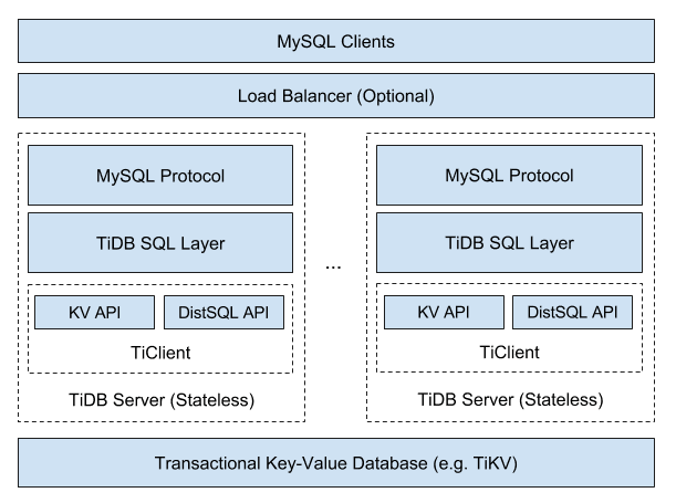
As you can see, TiDB is a SQL engine that supports the MySQL protocol with some kind of distributed KV storage engine that supports transactions as the underlying storage.
Here come three significant questions.
- How to support MySQL protocol?
- How to communicate with storage engine, store and load data?
- How to implement SQL functions?
This section will start with a few of brief descriptions of what modules TiDB has and what they do, and then put them together to answer these three questions.
Code Structure
TiDB source code is fully hosted on Github, you can see all the information from the repository homepage. The whole repository is developed in Golang and divided into many packages according to functional modules.
Most of the packages export services in the form of interfaces, and most of the functionality is concentrated in one package. But there are packages that provide basic functionality and are dependent on many packages, so these packages need special attention.
The main method of TiDB locates in tidb-server/main.go, which defines how the service is started.
The build system of the entire project can be found in the Makefile.
In addition to the code, there are many test cases, which can be found with suffix _test.go. There is also toolkit under the cmd directory for doing performance tests or constructing test data.
Module Structure
TiDB has a number of modules. Table below is an overview that shows what each module does, and if you want to see the code for the relevant function, you can find the corresponding module directly.
| Package | Description |
|---|---|
| pingcap/tidb/pkg/bindinfo | Handles all global sql bind operations, and caches the sql bind info from storage. |
| pingcap/tidb/pkg/config | The configuration definition. |
| pingcap/tidb/pkg/ddl | The execution logic of data definition language (DDL). |
| pingcap/tidb/pkg/distsql | The abstraction of the distributed computing interfaces to isolate the logic between the executor and the TiKV client |
| pingcap/tidb/pkg/domain | The abstraction of a storage space in which databases and tables can be created. Like namespace, databases with the same name can exist in different domains. In most cases, a single TiDB instance only creates one Domain instance with details about the information schema and statistics. |
| pingcap/tidb/pkg/errno | The definition of MySQL error code, error message, and error summary. |
| pingcap/tidb/pkg/executor | The operator related code that contains the execution logic of most statements. |
| pingcap/tidb/pkg/expression | The expression-related code that contains various operators and built-in functions. |
| pingcap/tidb/pkg/infoschema | The metadata management module for SQL statements; accessed when all the operations on the information schema are executed. |
| pingcap/tidb/pkg/kv | The Key-Value engine interface and some public methods; the interfaces defined in this package need to be implemented by the storage engine which is going to adapt TiDB SQL layer. |
| pingcap/tidb/pkg/lock | The implementation of LOCK/UNLOCK TABLES. |
| pingcap/tidb/pkg/meta | Manages the SQL metadata in the storage engine through the features of the structure package; infoschema and DDL use this module to access or modify the SQL metadata . |
| pingcap/tidb/pkg/meta/autoid | A module to generate the globally unique monotonically incremental IDs for each table, as well as the database ID and table ID. |
| pingcap/tidb/pkg/metrics | Store the metrics information of all modules. |
| pingcap/tidb/pkg/owner | Some tasks in the TiDB cluster can be executed by only one instance, such as the asynchronous schema change. This owner module is used to coordinate and generate a task executor among multiple TiDB servers. Each task has its own executor. |
| pingcap/tidb/pkg/parser | A MySQL compatible SQL parser used by TiDB, also contains the data structure definition of abstract syntax tree (AST) and other metadata. |
| pingcap/tidb/pkg/planner | Queries optimization related code. |
| pingcap/tidb/pkg/plugin | The plugin framework of TiDB. |
| pingcap/tidb/pkg/privilege | The management interface of user privileges. |
| pingcap/tidb/pkg/server | Code of the MySQL protocol and connection management. |
| pingcap/tidb/pkg/session | Code of session management. |
| pingcap/tidb/pkg/sessionctx/binloginfo | Output binlog information. |
| pingcap/tidb/pkg/sessionctx/stmtctx | Necessary information for the statement of a session during runtime. |
| pingcap/tidb/pkg/sessionctx/variable | System variable related code. |
| pingcap/tidb/pkg/statistics | Code of table statistics. |
| pingcap/tidb/pkg/store | Storage engine drivers, wrapping Key-Value client to meet the requirements of TiDB. |
| tikv/client-go | The Go client of TiKV. |
| pingcap/tidb/pkg/structure | The structured API defined on the Transactional Key-Value API, providing structures like List, Queue, and HashMap. |
| pingcap/tidb/pkg/table | The abstraction of Table in SQL. |
| pingcap/tidb/pkg/tablecodec | Encode and decode data from SQL to Key-Value. See the codec package for the specific encoding and decoding solution for each data type. |
| pingcap/tidb/pkg/telemetry | Code of telemetry collect and report. |
| pingcap/tidb/cmd/tidb-server | The main method of the TiDB service. |
| pingcap/tidb/pkg/types | All the type related code, including the definition of and operation on types. |
| pingcap/tidb/pkg/util | Utilities. |
At a glance, TiDB has 80 packages, which might let you feel overwhelmed, but not all of them are important, and some features only involve a small number of packages, so where to start to look at the source code depends on the purpose of looking at the source code.
If you want to understand the implementation details of a specific feature, then you can refer to the module description above and just find the corresponding module.
If you want to have a comprehensive understanding of the source code, then you can start from tidb-server/main.go and see how tidb-server starts and how it waits for and handles user requests. Then follow the code all the way through to see the exact execution of the SQL. There are also some important modules that need to be looked at to know how they are implemented. For the auxiliary modules, you can look at them selectively to get a general impression.
SQL Layer Architecture
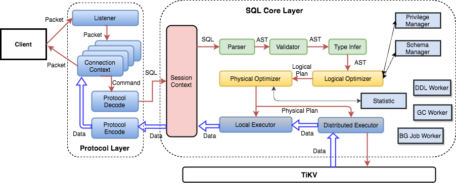
This is a detailed SQL layer architecture graph. You can read it from left to right.
Protocol Layer
The leftmost is the Protocol Layer of TiDB, this is the interface to interact with Client, currently TiDB only supports MySQL protocol, the related code is in the server package.
The purpose of this layer is to manage the client connection, parse MySQL commands and return the execution result. The specific implementation is according to MySQL protocol, you can refer to MySQL Client/Server Protocol document. If you need to use MySQL protocol parsing and processing functions in your project, you can refer to this module.
The logic for connection establishment is in the Run() method of server.go, mainly in the following two lines.
conn, err := s.listener.Accept()
clientConn := s.newConn(conn)
go s.onConn(clientConn)
The entry method for a single session processing command is to call the dispatch method of the clientConn class, where the protocol is parsed and passed to a different handler.
SQL Layer
Generally speaking, a SQL statement needs to go through a series of processes:
- syntax parsing
- validity verification
- building query plan
- optimizing query plan
- generating executor according to plan
- executing and returning results
These processes locate at the following modules:
| Package | Usage |
|---|---|
| pingcap/tidb/server | Interface between protocol layer and SQL layer |
| pingcap/tidb/parser | SQL parsing and syntax analyze |
| pingcap/tidb/planner | Validation, query plan building, query plan optimizing |
| pingcap/tidb/executor | Executor generation and execution |
| pingcap/tidb/distsql | Send request to TiKV and aggregate return results from TiKV via TiKV Client |
| pingcap/tidb/kv | KV client interface |
| tikv/client-go | TiKV Go Client |
KV API Layer
TiDB relies on the underlying storage engine to store and load data. It does not rely on a specific storage engine (such as TiKV), but has some requirements for the storage engine, and any engine that meets these requirements can be used (TiKV is the most suitable one).
The most basic requirement is "Key-Value engine with transactions and Golang driver". The more advanced requirement is "support for distributed computation interface", so that TiDB can push some computation requests down to the storage engine.
These requirements can be found in the interfaces of the kv package, and the storage engine needs to provide a Golang driver that implements these interfaces, which TiDB then uses to manipulate the underlying data.
As for the most basic requirement, these interfaces are related:
Transaction: Basic manipulation of transactionReceiver: Interface for reading dataMutator: Interface for mutating dataStorage: Basic functionality provided by the driverSnapshot: Basic manipulation of data snapshotIterator: Result ofSeek, used to iterate data
With the above interfaces, you are able to do all the required operations on the data and complete all the SQL functions. However, for more efficient computing, we have also defined an advanced computing interface, which can focus on these three interfaces or structures:
Client: Send request to storage engineRequest: Payload of the requestResponse: Abstraction of result
Summary
This section talks about the source structure of TiDB and the architecture of three significant components. More details will be described in the later sections.
The Life cycle of a Statement
MySQL protocol package with command and statement string
After connecting and getting authenticated, the server is in a statement execution loop until the client is disconnected.
The dispatch function checks what kind of command was sent through the MySQL protocol and dispatches the matching function, like this snippet:
	switch cmd {
	// ...
	case mysql.ComQuit:
		return io.EOF
	case mysql.ComInitDB:
		if err := cc.useDB(ctx, dataStr); err != nil {
			return err
		}
		return cc.writeOK(ctx)
	case mysql.ComQuery: // Most frequently used command.
		return cc.handleQuery(ctx, dataStr)
	// ...
	}
Where mysql.ComQuery is routed to handleQuery, which handles all different non-prepared statements (some commands like change database/schema or ping are handled directly in the dispatch function).
TiDB keep the state between statements like sql_mode, transaction state etc. in the clientConn's sessionctx.Context struct.
The MySQL protocol is synchronous, and the typical execution flow revolves around a client sending a single query, and receiving an optional result set ending with an OK package containing the success flag and optional warnings/errors and possible metadata such as affected rows.
As shown here; it is possible that a client might send multiple queries in one mysql.ComQuery call, in which case the cc.ctx.Parse will return multiple results. However; this is not a common occurrence. By default, multiple statements in one mysql.ComQuery call is disabled for security reasons, like making sql injections like SELECT user FROM users WHERE id = ''/* sql injection */; INSERT INTO users VALUES (null, 'EvilUser'); -- '. Clients must explicitly enable the ClientMultiStatements protocol feature.
High level code for handling a query
Real types and function names, but only high level for less distraction by too much details
Further explanations below.
// handleQuery is the entry point for running client connection statements/queries
func (cc *clientConn) handleQuery(ctx context.Context, sql string) (error) {
	stmts, err := cc.ctx.Parse(ctx, sql)
	// ...
	for i, stmt := range stmts {
		retryable, err = cc.handleStmt(ctx, stmt, ...)
		// ...
	}
}

// handleStmt handles a single statement
func (cc *clientConn) handleStmt(ctx context.Context, stmt ast.StmtNode, ...) (bool, error) {
	resultSet, err := cc.ctx.ExecuteStmt(ctx, stmt)
	// ...
	retryable, err := cc.writeResultset(ctx, resultSet, ...)
	// ...
}

func (tc *TiDBContext) ExecuteStmt(ctx context.Context, stmt ast.StmtNode) (ResultSet, error) {
	resultSet, err := tc.Session.ExecuteStmt(ctx, stmt)
	// ...
	return resultSet, err
}

// ExecuteStmt takes an Abstract Syntax Tree and will go through the optimizer and start the execution
// and return a recordSet.
func (s *session) ExecuteStmt(ctx context.Context, stmtNode ast.StmtNode) (sqlexec.RecordSet, error) {
	// ...
	compiler := executor.Compiler{Ctx: s}
	stmt, err := compiler.Compile(ctx, stmtNode)
	// ...
	resultSet, err := runStmt(ctx, s, stmt)
	// ...
	return resultSet, err
}

// Compile compiles an ast.StmtNode to a physical plan.
func (c *Compiler) Compile(ctx context.Context, stmtNode ast.StmtNode) (*ExecStmt, error) {
	// ...
	// PrepareTxnCtx starts a goroutine to begin a transaction if needed, and creates a new transaction context.
	s.PrepareTxnCtx(ctx)

	// Preprocess resolves table names of the node, and checks some statements validation.
	err := plannercore.Preprocess(c.Ctx, stmtNode, plannercore.WithPreprocessorReturn(ret), plannercore.WithExecuteInfoSchemaUpdate(pe))
	// ...
	// Optimize does optimization and creates a Plan.
	// The node must be prepared first.
	finalPlan, names, err := planner.Optimize(ctx, c.Ctx, stmtNode, ret.InfoSchema)
}

// runStmt executes the sqlexec.Statement and commit or rollback the current transaction.
func runStmt(ctx context.Context, se *session, s sqlexec.Statement) (sqlexec.RecordSet, error) {
	rs, err := s.Exec(ctx)
	// ...
	return &execStmtResult{RecordSet: rs, ...}, err
}

// writeResultset iterates over the Resultset and sends it to the client connection.
func (cc *clientConn) writeResultset(ctx context.Context, rs ResultSet ...) (bool, error) {
	retryable, err = cc.writeChunks(ctx, rs, ...)
	// ...
	return false, cc.flush(ctx)
}

// writeChunks writes data from a Chunk, which filled data by a ResultSet, into a connection.
func (cc *clientConn) writeChunks(ctx context.Context, rs ResultSet ...) (bool, error) {
	req := rs.NewChunk()
	for {
		err := rs.Next(ctx, req)
		// ...
		rowCount := req.NumRows()
		if rowCount == 0 {
			break
		}
		cc.writePacket(...)
	}
	return false, cc.writeEOF(...)
}
Statement string to Abstract Syntax Tree
In handleQuery the statement string is parsed by the parser, that is a MySQL compatible parser parsing statements and returns an Abstract Syntax Tree (AST) representing the statement. See more in the parser section
Example of Abstract Syntax tree, the fragment of a WHERE clause `id` > 1 AND `value` = 'Second' looks like:
ast.BinaryOperationExpr{
  Op: opcode.LogicAnd,
  L:  ast.BinaryOperationExpr{
    Op: opcode.GT,
    L:  ast.ColumnName{Name: 'id'},
    R:  parser_driver.ValueExpr{i: 1}
  },
  R: ast.BinaryOperationExpr{
    Op: opcode.EQ,
    L:  ast.ColumnName{Name: 'value'},
    R:  parser_driver.ValueExpr{b: 'Second'}
  },
}
AST -> Physical execution plan
Then the statement in AST form is handled in handleStmt/ExecuteStmt where the Abstract Syntax Tree is compiled first to a logical plan and then to a physical execution plan, including optimizing the execution plan, through a cost based optimizer. There are several steps in this process, such as name resolution, transaction management, privilege checks, handling given hints, etc.
One important thing to note is the planner.TryFastPlan() function that checks if there is a shortcut for a PointGet plan, to avoid spending too much time in the optimizer for simple queries, like primary key lookups.
For deeper understanding, please read the planner section
Example of plan from a simple select:
tidb> explain select id, value from t where id > 1 and value = 'Second';
+--------------------------+---------+-----------+---------------+----------------------------------+
| id                       | estRows | task      | access object | operator info                    |
+--------------------------+---------+-----------+---------------+----------------------------------+
| TableReader_7            | 0.00    | root      |               | data:Selection_6                 |
| └─Selection_6            | 0.00    | cop[tikv] |               | eq(test.t.value, "Second")       |
|   └─TableRangeScan_5     | 1.00    | cop[tikv] | table:t       | range:(1,+inf], keep order:false |
+--------------------------+---------+-----------+---------------+----------------------------------+
Where TableReader_7 is the task which will run in TiDB, getting already filtered data from Selection_6 scheduled on the storage nodes (TiKV/TiFlash) directly connected to the storage nodes Table/index range scan task/coprocessor, TableRangeScan_5.
Executing the optimized plan
The optimized plan is executed through runStmt, which builds an executor from the plan and will return a record set or directly execute the statements in case no records will be returned, like INSERT/UPDATE/DELETE statements. Before returning the record set, the executor starts the execution by calling the Volcano inspired Open() API and the Next() API to retrieve the first chunk of data or execute the statement fully if no records are to be returned.
The executors are often including coprocessors as seen above, where tasks can be seen as stream processors and can be parallelized and delegated to storage nodes (TiKV/TiFlash).
For Data Manipulation Language statements, the changes are buffered in a transaction buffer on the TiDB node, which is different in how MySQL/InnoDB handles it (where the changes are done directly in the btrees and undone in case of rollback. More information in the DML section
Requests sent to TiKV/TiFlash coprocessors
During the execution different task are executed as coprocessors and delegated/pushed down to the storage nodes (TiKV/TiFlash) for both scaling and more optimized use of the cluster.
This way there is less data sent between TiDB nodes and TiKV/TiFlash nodes (only filtered and aggregated results) and the computation/load are distributed across several storage nodes.
Common coprocessors are: TableScan (simplest form no real optimisation), IndexScan (Range reads from index), Selection (Filter on condition, WHERE clause etc.), LIMIT (no more than N records), TopN (Order + Limit), Aggregation (GROUP BY)
// HandleStreamRequest handles the coprocessor stream request.
func (h *CoprocessorDAGHandler) HandleStreamRequest(ctx context.Context, req *coprocessor.Request, stream tikvpb.Tikv_CoprocessorStreamServer) error {
  e, err := h.buildDAGExecutor(req)
  err = e.Open(ctx)
  chk := newFirstChunk(e)
  for {
    chk.Reset()
    err = Next(ctx, e, chk)
    // ...
    if chk.NumRows() == 0 {
       return h.buildResponseAndSendToStream(chk, ...)
    }
  }
}
As seen above the Volcano inspired execution is iterating over chunks of data, not records one-by-one, which also allows for vectorization, which formats the chunk data so it can be processed as a vector instead of looping over each record and column one by one.
Sending the result back to the client
If the statement returns a record set, it is handled in writeChunks which loops over the record set's Next() until empty and then adds some context/metadata to the MySQL OK package and flushes the data back to the client.
Notice that things like error handling, tracing etc. are not explained in this page.
DDL - Data Definition Language / Schema change handling
A short introduction to TiDB's DDL
The design behind TiDB's DDL implementation can be read in the Online DDL design doc.
TiDB is a distributed database which needs to have a consistent view of all schemas across the whole cluster. To achieve this in a more asynchronous way, the system uses internal states where each single stage transition is done so that the old/previous stage is compatible with the new/current state, allowing different TiDB Nodes having different versions of the schema definition. All TiDB servers in a cluster shares at most two schema versions/states at the same time, so before moving to the next state change, all currently available TiDB servers needs to be synchronized with the current state.
The states used are defined in tidb/parser/model/model.go:
        // StateNone means this schema element is absent and can't be used.
        StateNone SchemaState = iota
        // StateDeleteOnly means we can only delete items for this schema element.
        StateDeleteOnly
        // StateWriteOnly means we can use any write operation on this schema element,
        // but outer can't read the changed data.
        StateWriteOnly
        // StateWriteReorganization means we are re-organizing whole data after write only state.
        StateWriteReorganization
        // StateDeleteReorganization means we are re-organizing whole data after delete only state.
        StateDeleteReorganization
        // StatePublic means this schema element is ok for all write and read operations.
        StatePublic
Note: this is a very different implementation from MySQL, which uses Meta Data Locks (MDL) for keeping a single version of the MySQL instance schemas at a time. This results in MySQL replicas can have different version of the schemas, due to lag in asynchronous replication. TiDB has always a consistent view of all schemas in the cluster.
Implementation
All DDL jobs goes through two cluster wide DDL Queues:
- Generic queue for non data changes, DefaultJobListKey.
- Add Index Queue for data changes/reorganizations, AddIndexJobListKey, to not block DDLs that does not require data reorganization/backfilling).
The two base operations for these queue are:
- enqueue, adding one DDL job to the end of the queue.
- dequeue, pop the first DDL job from the queue (removing it from the queue and returning it).
When a DDL job is completed it will be moved to the DDL history.
There are two main execution parts handling DDLs:
- TiDB session, which executes your statements. This will parse and validate the SQL DDL statement, create a DDL job, and enqueue it in the corresponding queue. It will then monitor the DDL History until the operation is complete (succeeded or failed) and return the result back to the MySQL client.
- DDL background goroutines:
- limitDDLJobs which takes tasks from the sessions and adds to the DDL queues in batches.
- workers for processing DDLs:
- General worker, handling the default DDL queue where only metadata changes are needed.
- Add Index worker, which updates/backfills data requested in the AddIndexJob queue.
- DDL owner manager managing that one and only one TiDB node in the cluster is the DDL manager.
Execution in the TiDB session
The execution of the DDL is started through the 'Next' iterator of the DDLExec class (just like normal query execution):
 0  0x0000000003cd6cd5 in github.com/pingcap/tidb/executor.(*DDLExec).Next
    at ./executor/ddl.go:90
 1  0x0000000003cf3034 in github.com/pingcap/tidb/executor.Next
    at ./executor/executor.go:286
 2  0x0000000003c1f085 in github.com/pingcap/tidb/executor.(*ExecStmt).handleNoDelayExecutor
    at ./executor/adapter.go:584
 3  0x0000000003c1d890 in github.com/pingcap/tidb/executor.(*ExecStmt).handleNoDelay
    at ./executor/adapter.go:465
 4  0x0000000003c1d11e in github.com/pingcap/tidb/executor.(*ExecStmt).Exec
    at ./executor/adapter.go:414
 5  0x0000000003eedb56 in github.com/pingcap/tidb/session.runStmt
    at ./session/session.go:1682
 6  0x0000000003eec639 in github.com/pingcap/tidb/session.(*session).ExecuteStmt
    at ./session/session.go:1576
 7  0x0000000003fab0af in github.com/pingcap/tidb/server.(*TiDBContext).ExecuteStmt
    at ./server/driver_tidb.go:219
 8  0x0000000003f9c785 in github.com/pingcap/tidb/server.(*clientConn).handleStmt
    at ./server/conn.go:1841
 9  0x0000000003f9a5f2 in github.com/pingcap/tidb/server.(*clientConn).handleQuery
    at ./server/conn.go:1710
10  0x0000000003f94f9c in github.com/pingcap/tidb/server.(*clientConn).dispatch
    at ./server/conn.go:1222
11  0x0000000003f9133f in github.com/pingcap/tidb/server.(*clientConn).Run
    at ./server/conn.go:979
12  0x0000000003fd5798 in github.com/pingcap/tidb/server.(*Server).onConn
    at ./server/server.go:536
13  0x00000000012c4dc1 in runtime.goexit
    at /usr/lib/go-1.16/src/runtime/asm_amd64.s:1371
Where the different DDL operations are executed as their own functions, like:
        switch x := e.stmt.(type) {
        case *ast.AlterDatabaseStmt:
                err = e.executeAlterDatabase(x)
        case *ast.AlterTableStmt:
                err = e.executeAlterTable(ctx, x)
        case *ast.CreateIndexStmt:
                err = e.executeCreateIndex(x)
        case *ast.CreateDatabaseStmt:
                err = e.executeCreateDatabase(x)
        case *ast.CreateTableStmt:
                err = e.executeCreateTable(x)
        case *ast.CreateViewStmt:
                err = e.executeCreateView(x)
        case *ast.DropIndexStmt:
                err = e.executeDropIndex(x)
        case *ast.DropDatabaseStmt:
                err = e.executeDropDatabase(x)
Let us use the simple CREATE TABLE as an example (which does not need any of the WriteOnly or DeleteOnly states):
CREATE TABLE t (id int unsigned NOT NULL PRIMARY KEY, notes varchar(255));
This statement has the CreateTableStmt Abstract Syntax Tree type and will be handled by executeCreateTable/CreateTable functions.
It will fill in a TableInfo struct according to the table definition in the statement and create a DDL job and call doDDLJob which goes through the limitDDLJobs goroutine and adds one or more jobs to the DDL job queue in addBatchDDLJobs
DDL job encoded as JSON:
{
  "id": 56,
  "type": 3,
  "schema_id": 1,
  "table_id": 55,
  "schema_name": "test",
  "state": 0,
  "err": null,
  "err_count": 0,
  "row_count": 0,
  "raw_args": [
    {
      "id": 55,
      "name": {
        "O": "t",
        "L": "t"
      },
      "charset": "utf8mb4",
      "collate": "utf8mb4_bin",
      "cols": [
        {
          "id": 1,
          "name": {
            "O": "id",
            "L": "id"
          },
          "offset": 0,
          "origin_default": null,
          "origin_default_bit": null,
          "default": null,
          "default_bit": null,
          "default_is_expr": false,
          "generated_expr_string": "",
          "generated_stored": false,
          "dependences": null,
          "type": {
            "Tp": 3,
            "Flag": 4131,
            "Flen": 10,
            "Decimal": 0,
            "Charset": "binary",
            "Collate": "binary",
            "Elems": null
          },
          "state": 5,
          "comment": "",
          "hidden": false,
          "change_state_info": null,
          "version": 2
        },
        {
          "id": 2,
          "name": {
            "O": "notes",
            "L": "notes"
          },
          "offset": 1,
          "origin_default": null,
          "origin_default_bit": null,
          "default": null,
          "default_bit": null,
          "default_is_expr": false,
          "generated_expr_string": "",
          "generated_stored": false,
          "dependences": null,
          "type": {
            "Tp": 15,
            "Flag": 0,
            "Flen": 255,
            "Decimal": 0,
            "Charset": "utf8mb4",
            "Collate": "utf8mb4_bin",
            "Elems": null
          },
          "state": 5,
          "comment": "",
          "hidden": false,
          "change_state_info": null,
          "version": 2
        }
      ],
      "index_info": null,
      "constraint_info": null,
      "fk_info": null,
      "state": 0,
      "pk_is_handle": true,
      "is_common_handle": false,
      "common_handle_version": 0,
      "comment": "",
      "auto_inc_id": 0,
      "auto_id_cache": 0,
      "auto_rand_id": 0,
      "max_col_id": 2,
      "max_idx_id": 0,
      "max_cst_id": 0,
      "update_timestamp": 0,
      "ShardRowIDBits": 0,
      "max_shard_row_id_bits": 0,
      "auto_random_bits": 0,
      "pre_split_regions": 0,
      "partition": null,
      "compression": "",
      "view": null,
      "sequence": null,
      "Lock": null,
      "version": 4,
      "tiflash_replica": null,
      "is_columnar": false,
      "temp_table_type": 0,
      "policy_ref_info": null,
      "placement_settings": null
    }
  ],
  "schema_state": 0,
  "snapshot_ver": 0,
  "real_start_ts": 0,
  "start_ts": 428310284267159550,
  "dependency_id": 0,
  "query": "CREATE TABLE t (id int unsigned NOT NULL PRIMARY KEY, notes varchar(255))",
  "binlog": {
    "SchemaVersion": 0,
    "DBInfo": null,
    "TableInfo": null,
    "FinishedTS": 0
  },
  "version": 1,
  "reorg_meta": null,
  "multi_schema_info": null,
  "priority": 0
}
Execution in the TiDB DDL Owner
When the tidb-server starts, it will initialize a domain where it creates a DDL object and calls ddl.Start() which starts the limitDDLJobs goroutine and the two DDL workers. It also starts the CampaignOwner/campaignLoop which monitor the owner election and makes sure to elect a new owner when needed.
A ddl worker goes through this workflow in a loop (which may handle one job state per loop, leaving other work to a new loop):
- Wait for either a signal from local sessions, global changes through PD or a ticker (2 * lease time or max 1 second) and then calls handleDDLJobQueue.
- Start a transaction.
- Checks if it is the owner (and if not just returns).
- Picks the first job from its DDL queue.
- Waits for dependent jobs (like reorganizations/backfill needs to wait for its meta-data jobs to be finished first, which it is dependent on).
- Waits for the current/old schema version to be globally synchronized, if needed, by waiting until the lease time is passed or all tidb nodes have updated their schema version.
- If the job is done (completed or rolled back):
- Clean up old physical tables or indexes, not part of the new table.
- Remove the job from the ddl queue.
- Add the job to the DDL History.
- Return from handleDDLJobQueue, we are finished!
- Otherwise, execute the actual DDL job, runDDLJob See more about this below!
- Update the DDL Job in the queue, for the next loop/transaction.
- Write to the binlog.
The execution of the job's DDL changes in runDDLJob looks like this:
        // For every type, `schema/table` modification and `job` modification are conducted
        // in the one kv transaction. The `schema/table` modification can be always discarded
        // by kv reset when meets a unhandled error, but the `job` modification can't.
        // So make sure job state and args change is after all other checks or make sure these
        // change has no effect when retrying it.
        switch job.Type {
        case model.ActionCreateSchema:
                ver, err = onCreateSchema(d, t, job)
        case model.ActionModifySchemaCharsetAndCollate:
                ver, err = onModifySchemaCharsetAndCollate(t, job)
        case model.ActionDropSchema:
                ver, err = onDropSchema(d, t, job)
        case model.ActionCreateTable:
                ver, err = onCreateTable(d, t, job)
        case model.ActionCreateView:
                ver, err = onCreateView(d, t, job)
        case model.ActionDropTable, model.ActionDropView, model.ActionDropSequence:
                ver, err = onDropTableOrView(d, t, job)
        case model.ActionDropTablePartition:
                ver, err = w.onDropTablePartition(d, t, job)
        case model.ActionAddColumn:
                ver, err = onAddColumn(d, t, job)
        case model.ActionAddColumns:
                ver, err = onAddColumns(d, t, job)
        case model.ActionDropColumn:
                ver, err = onDropColumn(t, job)
        case model.ActionDropColumns:
                ver, err = onDropColumns(t, job)
        case model.ActionModifyColumn:
                ver, err = w.onModifyColumn(d, t, job)
        case model.ActionSetDefaultValue:
                ver, err = onSetDefaultValue(t, job)
        case model.ActionAddIndex:
                ver, err = w.onCreateIndex(d, t, job, false)
        case model.ActionDropIndex, model.ActionDropPrimaryKey:
                ver, err = onDropIndex(t, job)
        case model.ActionDropIndexes:
                ver, err = onDropIndexes(t, job)
        case model.ActionTruncateTable:
                ver, err = onTruncateTable(d, t, job)
        ...
Where each operation is handled separately, which is also one of the reasons TiDB has the limitation of only one DDL operation at a time (i.e. not possible to add one column and drop another column in the same DDL statement).
Following the example of CREATE TABLE we see it will be handled by onCreateTable, which after some checks, will create a new Schema version and if table is not yet in StatePublic state, it will create the table in CreateTableOrView which simply writes the TableInfo as a JSON into the meta database.
Notice that it will take another loop in the handleDDLJobQueue above to finish the DDL Job by updating the Schema version and synchronizing it with other TiDB nodes.
Graphs over DDL life cycle
An overview of the DDL execution flow in the TiDB cluster can be seen here:
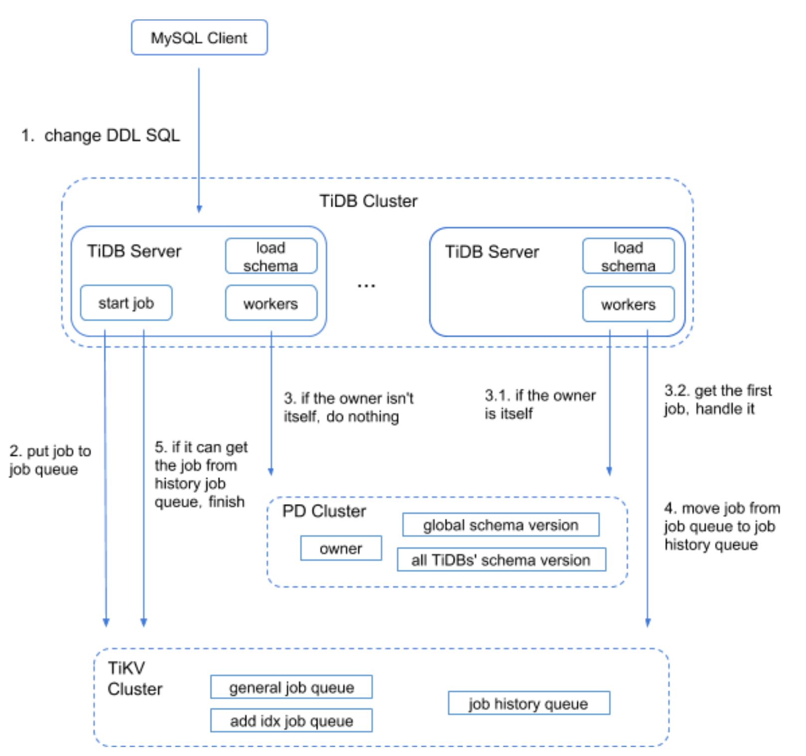
And more specifically for the DDL worker:
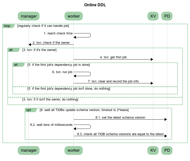
References
DML
Overview
DML is a sublanguage of SQL which is used as data manipulation. This document talks about the DML processing in TiDB.
This document refers to the code of TiDB v5.2.1 and TiKV v5.2.1.
Execution Process
The lifecycle chapter explains how queries are handled in TiDB. Different from DQLs which may write a lot of content to the client and should be processed in a streaming-like way, DMLs only report the result statistics(count of rows affected and inserted), which are handled by handleNoDelay function.
Generally, a DML statement is converted into delta changes in the execution process. When a transaction is committed, the changes will be applied atomically. Without starting a transaction explicitly, it'll be committed automatically. In which, this document focuses on how a DML is executed only.
Compare with DQLs, DMLs are relatively simple in optimization, it's easy to imagine how the delete, insert, update, and replace statements look like and how they should be executed. There may be some data sources in DMLs, like insert into table1 select from table2 which will insert the data from table2 into table1, however, you may not care about the data sources too much, since the data can be read by just calling Next of reading executors.
Like DQLs, the physical plans will be built into executors after optimization in the build function. The replace statement is treated as a kind of insert statement.
#![allow(unused)]
fn main() {
func (b *executorBuilder) build(p plannercore.Plan) Executor {
	switch v := p.(type) {
	case nil:
		return nil
	...
	case *plannercore.Delete:
		return b.buildDelete(v)
	...
	case *plannercore.Insert:
		return b.buildInsert(v)
	...
	case *plannercore.Update:
		return b.buildUpdate(v)
	...
	}
}
}
After the execution, the input SQL statements will be converted into delta changes and stored in MemDB, we'll talk about it later.
Like DQLs, DMLs also rely on the schema. When a SQL is compiled, the schema is assigned. Manipulating data should base on the corresponding schema. Tables in the schema offer Table interface, which is a medium of data manipulation.
Conflict
Without conflicts, DMLs are easy, they are converted into delta changes and waiting to be committed during execution. This section will talk about the conflict handle issue.
Optimistic
TiDB can check the conflict for optimistic transactions whether during execution and commit. The behavior is controlled by tidb_constraint_check_in_place. By default, TiDB won't check if there is a conflict when executing optimistic transactions. A conflict means that there is a record whose commit_ts is less than the current transaction's start_ts, by checking this situation TiDB needs to look up TiKV and see if such a record exists, there the latency is introduced. The code for handling the row key and unique index key is below.
// AddRecord implements table.Table AddRecord interface.
func (t *TableCommon) AddRecord(sctx sessionctx.Context, r []types.Datum, opts ...table.AddRecordOption) (recordID kv.Handle, err error) {
		...
		} else if sctx.GetSessionVars().LazyCheckKeyNotExists() {
			var v []byte
			v, err = txn.GetMemBuffer().Get(ctx, key)
			if err != nil {
				setPresume = true
			}
			if err == nil && len(v) == 0 {
				err = kv.ErrNotExist
			}
		} else {
			_, err = txn.Get(ctx, key)
		}
		...
}

// Create creates a new entry in the kvIndex data.
// If the index is unique and there is an existing entry with the same key,
// Create will return the existing entry's handle as the first return value, ErrKeyExists as the second return value.
func (c *index) Create(sctx sessionctx.Context, txn kv.Transaction, indexedValues []types.Datum, h kv.Handle, handleRestoreData []types.Datum, opts ...table.CreateIdxOptFunc) (kv.Handle, error) {
...
	} else if sctx.GetSessionVars().LazyCheckKeyNotExists() {
		value, err = txn.GetMemBuffer().Get(ctx, key)
	} else {
		value, err = txn.Get(ctx, key)
	}
...
}
Skipping checking the existence of records reduces latency, and if there is such a record, the optimistic transactions will suffer an error when committing. In the prewrite phase, if there is a record whose commit_ts is less than self's start_ts, an already-exist error will be returned and the current transaction should abort, so there are no correctness issues.
As for the use case which requires checking if the key exists in execution, just turn tidb_constraint_check_in_place on.
Pessimistic
Since optimistic transactions check if can submit in prewrite phases, in a high contention use case, there may be cascade abort, and the fail rate of the transaction will increase rapidly. Further, aborted transactions need to be cleaned up, as a result, many resources are wasted.
As the image shows, pessimistic transactions go through a 2PL way.
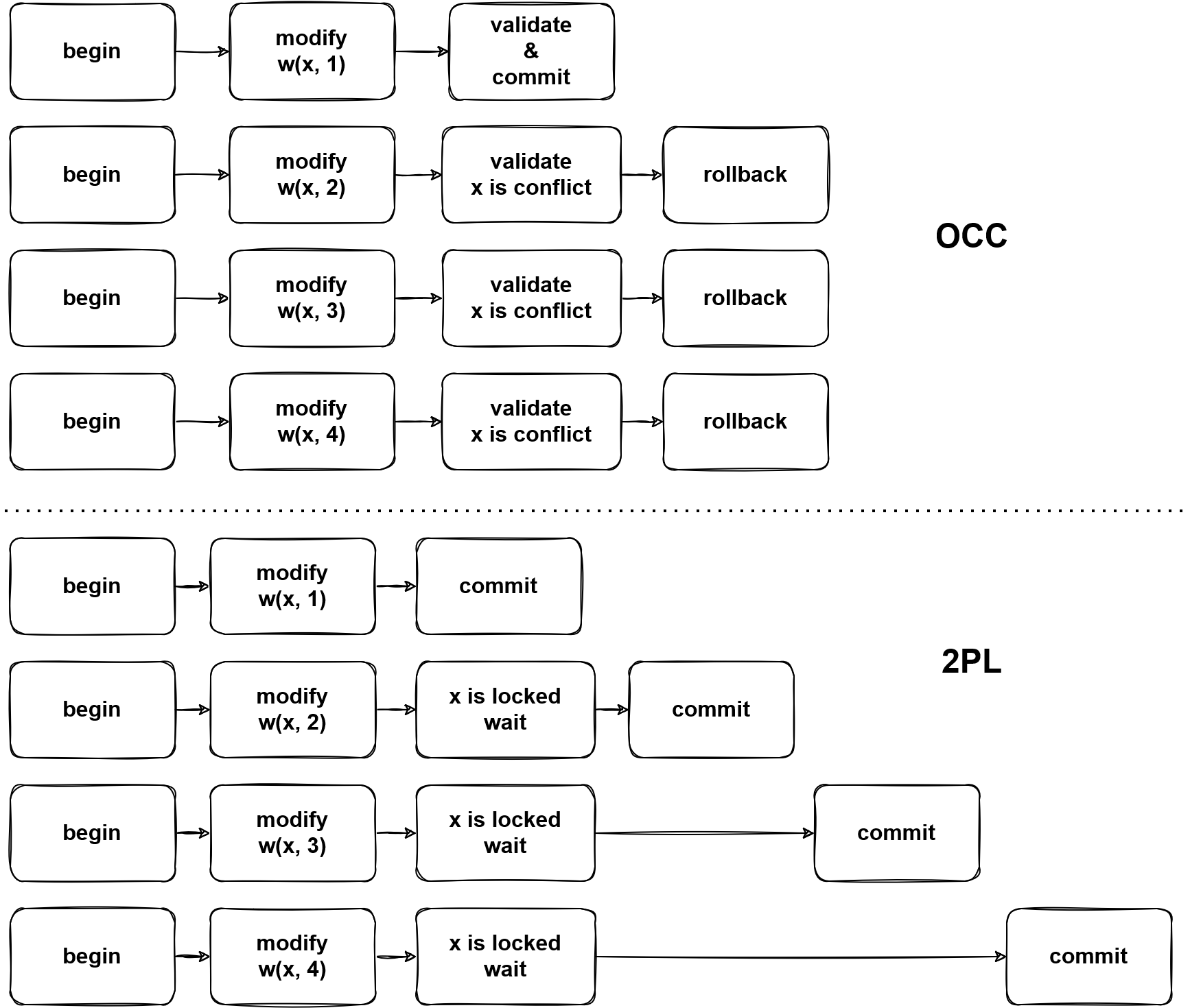
By any write operations, the corresponding pessimistic locks will be written into TiKV, then other transactions which tend to modify the locked data, a key is locked error will be returned from TiKV, then TiDB will block the statement until the lock is cleared or expired.
The pessimistic transaction lock key is in two steps, e.g. UPDATE t SET v = v + 1 WHERE id < 10:
- Read the required data from TiKV, it's like
SELECT row_id FROM t WHERE id < 10got (1, 1), (2, 4). - Now TiDB knows which key exists, then based on the read data, lock keys.
However, there is a specific way to add a pessimistic, aka. lock and read in the same time. It's an atomic operation, read keys from TiKV and the result is returned with keys locked. Luckily, this way is not widely used, only in point_get and batch_point_get. This operation will lock the not-exist keys, which allows the client to lock keys first and write some values later. TiDB handles this case by adding the KVs to a pessimistic lock cache after pessimistic lock is done.
There is a special read which is different from snapshot read, which read the data from the latest snapshot. We can call it current read or for-update read. In snapshot isolation, all statements in a transaction are executed in the same snapshot, so there are no non-repeatable or non-phantom reads. However, write operations in pessimistic transactions should affect the latest version of data, which means that they use the different snapshot from the read snapshot.
MemDB
The delta changes are stored in MemDB in TiDB until the transaction is committed. MemDB is an ordered in-memory storage(implemented in the red-black tree) with the following requirements.
- Revert changes.
- Flag support.
Think about an in-transaction statement get failed because of conflict or constraint violation, then an error is reported to the client, this statement should take no effect. However, there may already be some changes are written to the MemDB before encountering the error. These changes need to be reverted. In TiDB, StmtCommit handles the statement level commit which will flush the changes of successful statements from the staging buffer into MemDB. Here are the key methods of the MemBuffer interface.
// MemBuffer is an in-memory kv collection, can be used to buffer write operations.
type MemBuffer interface {
	...
	// Staging create a new staging buffer inside the MemBuffer.
	// Subsequent writes will be temporarily stored in this new staging buffer.
	// When you think all modifications looks good, you can call `Release` to public all of them to the upper level buffer.
	Staging() StagingHandle
	// Release publish all modifications in the latest staging buffer to upper level.
	Release(StagingHandle)
	// Cleanup cleanup the resources referenced by the StagingHandle.
	// If the changes are not published by `Release`, they will be discarded.
	Cleanup(StagingHandle)
	...
}
The KeyFlags are the metadata of keys, they mark the keys with states. You can learn the meaning from their names, e.g. if flagPresumeKNE is set, the key is presumed as not existing in TiKV, which means this is an inserted key, otherwise, it's an updated key.
Summary
This document talks about DML generally. However, TiDB is a complex system, and DML has correlation with most components, you may be confused about many details with manipulation of data, reading other documents or the source code would make it clear.
DQL
Overview
This chapter describes the execution process of a data query statement in TiDB. Starting from the SQL processing flow, it describes how a SQL statement is sent to TiDB, how TiDB processes it after receiving the SQL statement, and how the execution result is returned.
Execution Process
Briefly, the execution process of a SQL statement can be divided into three stages:
-
Protocol Layer
Protocol layer is responsible for parsing the network protocol. Its code locates at
serverpackage, mainly consisting of two parts: one for connection establishing and management, every connection corresponds to one session separately; one for handling the packets read from the connection. -
SQL Layer
SQL layer is the most complex part in TiDB, handling SQL statement parsing and execution. SQL is a complex language, having various data types and operators, numerous syntax combinations. Besides, TiDB uses a distributed storage engine underneath, so it will encounter many problems standalone storage engines won't.
-
KV API Layer
KV API layer routes requests to the right KV server and passes the results back to SQL layer. It should handle the exceptions happened in this stage.
A SQL statement goes through the above three stages sequentially, get parsed and transformed, then handled by SQL layer. In SQL layer, query plans are generated and executed, retrieving data from the underneath storage engine. We'll give a detailed introduction to SQL layer.
Protocol Layer
Entry
The entry of TiDB's SQL layer is in server/conn.go. After a connection is established between the client and TiDB, TiDB spawns a goroutine to listen and poll on the port. In clientConn.Run(), a loop keeps reading network packets and calls clientConn.dispatch() to handle them:
data, err := cc.readPacket()
if err = cc.dispatch(ctx, data)
dispatch handles the raw data array. The first byte of the array represents command type. Among the types, COM_QUERY represents data query statement. You can refer to MySQL protocol for more information about the data array. For COM_QUERY, its content is SQL statement. clientConn.handleQuery() handles the SQL statement. It calls TiDBContext.ExecuteStmt() in server/driver_tidb.go:
func (tc *TiDBContext) ExecuteStmt(ctx context.Context, stmt ast.StmtNode) (ResultSet, error) {
	rs, err := tc.Session.ExecuteStmt(ctx, stmt)
session.ExecuteStmt() is the entry of the SQL layer kernel and returns the result of the SQL execution.
Exit
After a series of operations described above, the execution results will be returned to the client in COM_QUERY response format by clientConn.writeResultSet().
SQL Layer
In SQL layer, there are multiple concepts and interfaces we need to pay close attention to:
Session
The most important function in Session is ExecuteStmt. It wraps calls to other modules. The SQL execution will respect environment variables in Session like AutoCommit and timezone.
Parser
Parser consists of Lexer and Yacc. It turns the SQL text to AST:
p := parserPool.Get().(*parser.Parser)
defer parserPool.Put(p)
p.SetSQLMode(s.sessionVars.SQLMode)
p.SetParserConfig(s.sessionVars.BuildParserConfig())
tmp, warn, err := p.Parse(sql, charset, collation)
In the parsing process, lexer first transforms the SQL text to tokens, and then parser accepts the tokens as inputs and generates appropriate AST nodes. For example, statement SELECT * FROM t WHERE c > 1; matches SelectStmt rule finally turns to the structure below:
type SelectStmt struct {
	dmlNode
	// SelectStmtOpts wraps around select hints and switches.
	*SelectStmtOpts
	// Distinct represents whether the select has distinct option.
	Distinct bool
	// From is the from clause of the query.
	From *TableRefsClause
	// Where is the where clause in select statement.
	Where ExprNode
	// Fields is the select expression list.
	Fields *FieldList
	// GroupBy is the group by expression list.
	GroupBy *GroupByClause
	// Having is the having condition.
	Having *HavingClause
	// WindowSpecs is the window specification list.
	WindowSpecs []WindowSpec
	// OrderBy is the ordering expression list.
	OrderBy *OrderByClause
	// Limit is the limit clause.
	Limit *Limit
	// LockInfo is the lock type
	LockInfo *SelectLockInfo
	// TableHints represents the table level Optimizer Hint for join type
	TableHints []*TableOptimizerHint
	// IsInBraces indicates whether it's a stmt in brace.
	IsInBraces bool
	// WithBeforeBraces indicates whether stmt's with clause is before the brace.
	// It's used to distinguish (with xxx select xxx) and with xxx (select xxx)
	WithBeforeBraces bool
	// QueryBlockOffset indicates the order of this SelectStmt if counted from left to right in the sql text.
	QueryBlockOffset int
	// SelectIntoOpt is the select-into option.
	SelectIntoOpt *SelectIntoOption
	// AfterSetOperator indicates the SelectStmt after which type of set operator
	AfterSetOperator *SetOprType
	// Kind refer to three kind of statement: SelectStmt, TableStmt and ValuesStmt
	Kind SelectStmtKind
	// Lists is filled only when Kind == SelectStmtKindValues
	Lists []*RowExpr
	With  *WithClause
}
From t is parsed to From field. WHERE c > 1 is parsed to Where field. * is parsed to Fields field. Most data structures in ast package implement ast.Node interface. This interface has a Accept method, implementing the classic visitor pattern, used by following procedures to traverse the tree.
Compile
After the AST is generated, it's going to be validated, transformed and optimized in Compiler.Compile():
compiler := executor.Compiler{Ctx: s}
stmt, err := compiler.Compile(ctx, stmtNode)
There are three steps:
plan.Preprocess: do validations and name binding.plan.Optimize: make and optimize query plans, this is the core part.- construct
executor.ExecStmtstructure: ExecStmt holds the query plans. It's the foundation for following execution.
Executor
While constructing the executor in ExecStmt.buildExecutor(), query plans are turned to executor. Then the execution engine could perform the query plans via the executor. The generated executor is encapsulated in a recordSet structure:
return &recordSet{
	executor:   e,
	stmt:       a,
	txnStartTS: txnStartTS,
}
This structure implements ast.RecordSet interface. It abstracts the query results and has the following methods:
type RecordSet interface {
	// Fields gets result fields.
	Fields() []*ast.ResultField
	// Next reads records into chunk.
	Next(ctx context.Context, req *chunk.Chunk) error
	// NewChunk create a chunk.
	NewChunk() *chunk.Chunk
	// Close closes the underlying iterator, call Next after Close will
	// restart the iteration.
	Close() error
}
The functionality of each method is described in the comments. In short, Fields() retrieves the type of each column. Next() returns a batch of the result. Close() closes the result set.
TiDB's execution engine executes in Volcano model. All the executors constitute an executor tree. Every upper layer gathers results from the lower layer by calling its Next() method. Assuming we have a SQL statement SELECT c1 FROM t WHERE c2 > 1; and the query plan is full table scanning plus filtering, the executor tree is like:
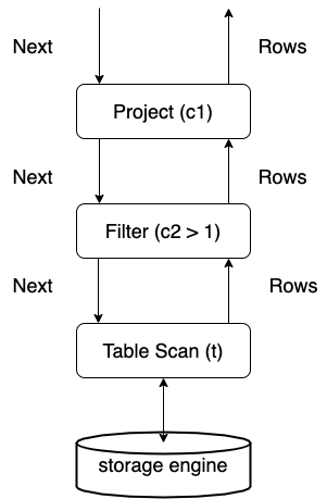
From the above picture, we can see the data flow between executors. The starting point of a SQL statement execution, also the first Next() call is in the function returning data back to the client:
err := rs.Next(ctx, req)
rs is a RecordSet instance. Keep calling its Next method to get more results to return to the client.
Overall Diagram
The above SQL query statement execution process can in general be described as the following picture:
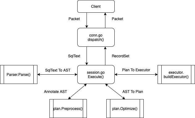
Parser
Parser is responsible for interpreting a SQL string into an abstract syntax tree (AST), which is more structural and easier to process. AST can be used for preprocessing, syntactic analysis, and so on.
The code lives in the pingcap/tidb repo, parser directory.
Understand Parser
Parser is generated by a parser generator named yacc. It takes the grammar file parser.y as the input and outputs the source code file parser.go, which is the real parser imported by TiDB. Thus, the core file is parser.y because when the SQL syntax changes, most of the changes take place in parser.y.
In case you are unfamiliar with yacc, some concepts are listed here:
- Terminal Symbol is also known as "token". When a SQL string reaches parser, the first step is to tokenize them into an array of tokens. For example,
"SELECT * FROM t"is tokenized to[selectKeyword, '*', fromKeyword, identifier(t)]by lexer.Lex(). - Non-terminal Symbol is a syntactic variable, which can represent a group of terminal/non-terminal symbols.
- Grammar Rule specifies which symbols can replace which other non-terminal symbol.
- Semantic Action defines how an AST node is constructed.
An example of a grammar rule is as follows:
AlterDatabaseStmt:
	"ALTER" DatabaseSym DBName DatabaseOptionList
	{
		$$ = &ast.AlterDatabaseStmt{
			Name:                 $3,
			AlterDefaultDatabase: false,
			Options:              $4.([]*ast.DatabaseOption),
		}
	}
AlterDatabaseStmtis a non-terminal symbol because there is no such token."ALTER"is a terminal symbol.DatabaseSym,DBNameandDatabaseOptionListare non-terminal symbols that are defined in other grammar rules.- The pseudo-code in brackets is the semantic action. It means an AST node
ast.AlterDatabaseStmtwill be constructed when the rule is reduced by the parser. Note that a dollar character$followed by a number represents the binding Golang value previously (in other rules), where the number is the index of symbol in rule (1-based).$$represents current binding value. After goyacc substitution, this code snippet will be valid Golang code.
Getting back to parser.y, the structure of this file is divided into three parts:
%unionenumerates all the Golang types that can be passed around grammar rules.%tokenor%typedeclares the terminal or non-terminal symbols that will be used in grammar rules.- Grammar rules define the syntax of SQL and related semantic actions.
Except for parser.y, other sub-package/files should be easy to understand, feel free to explore them by yourself:
| Package | Description |
|---|---|
| ast | The AST definition used by TiDB. |
| auth | Authentication-related functions. |
| charset | Currently supported charsets and encodings. |
| format | The Formatters for yacc file and the functions for restoring AST to SQL. |
| goyacc | The generator for parser.go. |
| model | Basic structures in TiDB like TableInfo, ColumnInfo... |
| mysql | MySQL constants, errors, privileges, types, and others. |
| opcode | Operator code like <, >, +, =... |
| terror | The errors used by TiDB. |
| test_driver | A parser driver only for unit tests. |
| tidb | TiDB related features' keywords. |
| types | The field types and evaluation types that used in TiDB. |
Develop and Build
To get started with the parser development, please also take a look at quickstart.md. It shows the basic usage of the parser and it explains some concepts like parser_driver.
Run make parser in the project root directory to generate a new parser.go.
FAQ
- How to debug the parsing procedure?
Put the test file in the parser package. Set yyDebug level to 4(or any integers >= 4) before calling Parse(). The parser will try to show state information in each step.
- How to resolve shift-reduce or reduce-reduce conflicts?
Shift means "move the next token in" to match the current rule. Reduce means "replace current tokens/symbols to a non-terminal symbol". Shift-reduce conflicts occur when the parser cannot decide the next step is to shift or to reduce.
When yacc reports such conflicts, it also keeps the file y.output. You can search "conflict on" in the file to locate which rule conflicts with other rules. Then you can try to annotate the %precedence to tokens, rewrite the grammar rule, or ask for help on GitHub.
Planner
The planner package contains most of the codes related to SQL optimization. The input of the planner is an AST of the query returned from the parser, and the output of the planner is a plan tree that would be used for further execution.
Package Structure
| Package | Description |
|---|---|
| tidb/pkg/planner/cascades | The next generation Cascades model planner, which is under development and disabled by default |
| tidb/pkg/planner/core | The core logic of the currently used System R model planner. The Cascades model planner also calls utility functions in this package |
| tidb/pkg/planner/implementation | Physical implementations for the operators in Cascades planner |
| tidb/pkg/planner/memo | Intermediate results for the searching procedure of Cascades planner |
| tidb/pkg/planner/property | Properties about the output of operators, including schema, stats, order property, partition property, etc |
| tidb/pkg/planner/util | Common utility functions / structures shared by the two planners |
We can see that, TiDB has two planners, one is of System R model, which is defaultly used, and the other is of Cascades model, which is still under development. The unified entry function of planner module is Optimize(), before diving into either of the two planners, it would firstly check if there is any intervention for the planner from the "SQL Plan Management" module, if yes, the AST of the query would be modified before going through the optimization procedures. "SQL Plan Management" module is beyond the scope of this article, and it would be introduced in the SQL Plan Management section.
This article would only focus on introducing the System R planner, i.e, the core package, readers who are interested in the Cascacdes planner can refer to this design doc.
Optimization Procedures
Ignore the trivial steps, the query optimization procedures can be briefly divided into 4 phases:
- build an initial logical plan
- logically optimize the initial logical plan
- physically optimize the logical plan
- tidy up the physical plan
Plan Building
The entry function of this phase is PlanBuilder.Build(), it would translate the input AST to a logical plan tree from bottom up according to the predefined rules / orders. Specifically, it would check each sub-clause of the query, and build a corresponding operator for the clause. The operators are connected as a DAG, which is known as a logical plan tree.
A key step in this phase is translating the expressions for each clause, e.g, where a = 1 would have a Selection operator built correspondingly, and an expression eq(a, 1) would be translated and saved in the Selection operator. The expression translation logics are encapsulated in a structure expressionRewriter and its methods. The expressionRewriter would traverse and transalte the AST expressions recursively, and utilize a result stack for intermediate results.
expressionRewriter would not only do the simple expression transaltions, but would optimize subqueries in the expressions. The details of subquery optimization would not be explained here, because they are pretty complicated. Briefly speaking, for most of the uncorrelated subqueries, expressionRewriter would directly execute them and substitute them with the result constants. For correlated subqueries, or some of the uncorrelated subqueries, expressionRewriter would build a subtree from them and connect it with the main plan tree using a LogicalJoin or LogicalApply operator. Note that, LogicalApply is a special kind of join operator which can only be executed in a nested-loop approach. LogicalApply operator in some plan trees can be converted to a regular LogicalJoin, which can be executed in other more efficient join algorithms, and planner would do this conversion in the subsequent logical optimization phase if possible.
During the plan building process, optimization flags would be collected for each operator built. For example, if a Selection operator is built, then an optimization flag like flagPredicatePushDown would be set in the plan builder. These saved flags would be used later in the logical optimization phase.
Logical Optimization
The entry function of this phase (also known as rule-based optimization) is logicalOptimize(). This function would do logically equivalent transformations for the initial plan tree according to relational algebra, and the result plan tree should be better than the initial one from the execution efficiency perspective in principle. Specifically, logicalOptimize() would traverse all the logical optimization rules predefined as optRuleList in order, and check if a rule is applicable by referring to the optimization flags saved during the plan building phase. If the flag is set for a rule, planner would traverse the plan tree from top down, and apply the transformations implied by the rule to the subtree satisfying the rule prerequisites.
An example logical optimization rule is "column pruning", for each operator in the plan tree, it would collect the columns needed by the upper operators, and prune the unneeded columns from the output. Another example rule is "decorrelation", it would try to pull up operators referring correlated columns, and resolve the column dependency, hence convert the LogicalApply operator to a regular LogicalJoin.
Physical Optimization
The entry function of this phase (also known as cost-based optimization) is physicalOptimize(), it would do cost based enumeration for the implementations of each logical operator, and find a combination of all operators with the lowest cost as the final physical plan. Specifically, each logical operator would implement an interface function exhaustPhysicalPlans() to list all the possible physical algorithms, e.g, LogicalAggregation would have two possible implementations including PhysicalStreamAggregation and PhysicalHashAggregation. Each implementation may require specific properties for its child's output, e.g, PhysicalStreamAggregation would require that the child's output rows should be in order of the GROUP BY columns. These properties are recorded in PhysicalProperty structure, and passed down to the enumeration procedure of the child operators.
Once the planner knows the specific implementation of the plan tree, or of a subtree, it can compute a cost for this implementation. The cost of one implementation is calculated as a sum of its resource consumptions including CPU, Memory, Network, IO, etc. For each kind of resource specifically, the consumption is measured based on a unit factor (e.g, scanFactor is the unit factor for IO consumption, which means the cost of scanning 1 byte data on TiKV or TiFlash), and the estimated number of rows / bytes to be processed by this operator. Note that, these unit factors can be customized by setting system variables like tidb_opt_xxx_factor to fit clusters of different hardware configurations. Each implementation of the whole logical plan tree would have a cost then, planner would choose the one with the lowest cost for execution.
One thing worth mention is that, TiDB supports pushing some operators down to storage engine to speed up the query execution, e.g, we can push Selection operator down to the coprocessor of TiKV, and reduce the rows returned from TiKV to TiDB through the network. The logic about deciding whether to push operators down to storage engine or not is piggybacked on the search framework of the physical optimization. Specifically, it is achieved by introducing TaskType field into PhysicalProperty, for example, once the planner wants to push down a Limit operator to TiKV, it would enumerate an implementation PhysicalLimit which has CopXXXTaskType as the TaskType of the required PhysicalProperty for its child. Once the child of PhysicalLimit has generated a TiKV implementation, these two plan snippets would be concatenated in attach2Task() interface, hence achieving the operator pushdown for storage engine.
Post Optimization
The entry function of this phase is postOptimize(). The query optimization has almost finished when coming here, this phase would not apply big changes to the plan, it would only do some clean and tidy up works. The jobs in this phase include a new round of projection elimination(the first round is applied in logical optimization), and projection injection to simplify the code implementations of executor package, and so on.
Summary
This section talks about the brief steps of query optimization, and the corresponding entry functions for each step.
Table Statistics
Like most commercial databases, TiDB query optimization incorporates a cost-based optimizer that relies on the statistics of the database data to make an optimal query plan. Therefore, the statistics play a key role in TiDB for the optimizer to choose, e.g., the right index for table access or the right join method between the index nested loop join and hash join, and many more scenarios for an optimal query execution plan.
In this chapter, we will introduce different types of statistics being used in TiDB, the corresponding data structure, how TiDB collects and maintains them, as well as how the TiDB optimizer uses these statistics in the optimization process. Given the space limit, we will not cover all the implementation details. However, the corresponding code modules will be pointed out as much as possible. Please also note that as TiDB and its optimizer evolve over time, some of these statistics and their application may also have evolved or been modified.
Types of TiDB statistics
Among many types of statistics commonly used by databases, TiDB mainly uses three types of them: histogram, top-n values (a.k.a, MFV or most frequent values), and count-min sketch (CM sketch). We will briefly introduce each of these statistics first.
Histogram
Histogram splits the data into a number of buckets and maintains some information to describe a bucket, such as the number of records in the bucket. It is widely used in many RDBMS to estimate a range.
Among two commonly used histogram strategies, equal-depth and equal-width, we choose the equal-depth histogram for it has a better guarantee of worst case error rate compared to that of the equal-width histogram. You can refer to the paper Accurate estimation of the number of tuples satisfying a condition for more information. With the equal-depth histogram, the number of values in each bucket is to be as equal as possible. For example, to split the given record set of 1.6, 1.9, 1.9, 2.0, 2.4, 2.6, 2.7, 2.7, 2.8, 2.9, 3.4, 3.5 into 4 buckets, the final buckets would look like [1.6, 1.9], [2.0, 2.6], [2.7, 2.8], [2.9, 3.5]. Thus the depth, (a.k.a. the number of records) of each bucket is 3, as shown in the following graph.
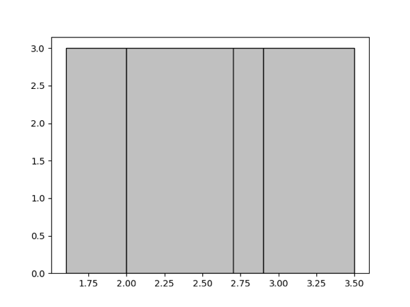
Count-Min Sketch
The Count-Min Sketch (CM sketch) is a data structure used for query cardinality estimation for the equal predicate, or join, etc., and provides strong accuracy guarantees. Since its introduction in 2003 in the paper An improved data stream summary: The count-min sketch and its applications, it has gained widespread use given its simplicity of construction and use.
CM sketch maintains an array of d*w counts, and for each value, maps it to a column in each row using d separate hash functions and modifies the count value at those d positions. This is shown in the following figure.
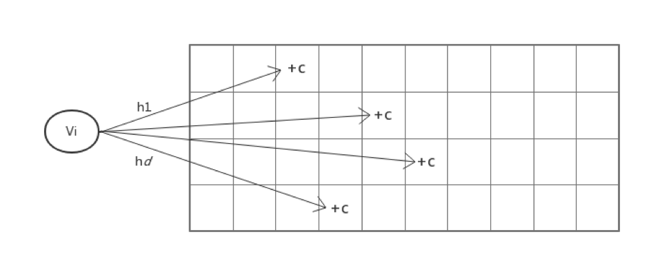
This way, when querying how many times a value appears, the d hash functions are still used to find the position mapped to in each row, and the minimum of these d values is used as the estimate.
Please note that CM sketch is not used as default statistics since version 5.1 given the increasing concerns on estimation bias under the scenarios with large distinct values of a column.
Top-N Value (Most Frequent Value)
The CM sketch would encounter severe hash collisions when the dataset grows while the histogram has its limit to estimate the selectivity of equal predicates. Thus we extract the Top-N value (a.k.a., the most frequent value) of the dataset out of the histogram to improve the accuracy of the estimation of an equal predicate. Here, the top-n statistics are stored as a pair of (value, cnt). For example, for a dataset 1, 1, 1, 1, 1, 1, 1, 2, 2, 3, 4, 4, 5, 6, 7. if n of top-n is 1, the top-n value pair will be [(1, 7)], and the rest of the histogram is constructed using the remaining data 2, 2, 3, 4, 4, 5, 6, 7. You may refer to the paper Synopses for Massive Data: Samples, Histograms, Wavelets, Sketches for additional information.
Statistics Construction
When the analyze command is executed, TiDB will collect the histogram, CM sketch, and top-n values statistics. During the execution of analyze command, the columns and indexes that need to be analyzed are divided into different tasks in builder.go, and then the tasks are pushed down to TiKV for execution in analyze.go. Here we will focus on the construction of histograms as an example.
Construction of column histogram
When constructing a column histogram, sampling will be performed first, and then the histogram will be constructed. The detailed steps are shown as follows.
In the collect function, we implemented the reservoir sampling algorithm to generate a uniform sampling set. Since its principle and code are relatively simple, it will not be introduced here.
After sampling, in BuildColumn, we implement the construction of column histogram. The samples are sorted first, then the height of each bucket is determined, and followed by traversing each value v sequentially:
- If
vis equal to the previous value, then putvin the same bucket as the previous value, regardless of whether the bucket is full or not so that each value can only exist in one bucket. - If it is not equal to the previous value, then check whether the current bucket is full. If bucket still has room to store a new item, put
vdirectly into the current bucket, and use updateLastBucket to change the upper bound and depth of the bucket.
- Otherwise, use AppendBucket to put in a new bucket.
You can find how we extract the top-n values then build the histogram in BuildHistAndTopN.
Construction of the indexed histogram
When constructing the index column histogram, we use SortedBuilder to maintain the intermediate state of the building process. Since the number of rows of data cannot be known in advance, the depth of each bucket cannot be determined. However, since the data in the index column is already ordered, we set the initial depth of each bucket to 1 in NewSortedBuilder. For each piece of data, Iterate will insert the data in a similar way when constructing a column histogram. If at a certain point, the number of required buckets exceeds the current bucket number, then use mergeBucket to merge every two previous buckets into one, double the bucket depth, and then continue to insert.
After collecting the histograms separately established on each Region, we also need to merge the histograms on each Region with MergeHistogram. In this function:
- In order to ensure that each value only appears in one bucket, we deal with the problem of the buckets at the junction, that is, if the upper and lower bounds of the two buckets at the junction are equal, then the two buckets need to be merged first;
- Before actual merging, we adjust the average bucket depth of the two histograms to be approximately equal;
- If the number of buckets exceeds the limit after the histogram is merged, then the two adjacent buckets are merged into one.
Statistics maintenance
From version 2.0, TiDB has introduced a dynamic update mechanism, which can dynamically adjust statistics based on the results of the query. In addition, from version 4.0, we have introduced the auto analyze function, which can automatically trigger the collection of (incremental) statistics based on the percentage of table data change.
As data changes significantly, the settings of statistics collection may need to be modified accordingly, too. For example, the histogram needs to adjust the bucket height and the boundaries of the bucket; and the CM Sketch needs to adjust the count array so that the estimated value is equal to the result of the query.
What needs to be pointed out here is that dynamically adjusting statistics based on query results is turned off by default in version 4.0, and will be revisited for a possible redesign in future versions.
The application of the statistics
Estimation
Query filtering conditions are often used in query statements to filter out certain data. Thus the main function to exploit statistics is to estimate the number of data after applying these filter conditions so that the optimizer may choose the optimal execution plan based on those estimates. We will introduce two main types of estimation for range and point filtering.
Range estimation
For a query that results in a range of data sets on a particular column, we choose the histogram for estimation.
In the previous introduction of the equal-depth histogram, an example of a histogram is given containing four buckets [1.6, 1.9], [2.0, 2.6], [2.7, 2.8], [2.9, 3.5], all of which have a bucket depth of 3. Suppose we have such a histogram, and we want to know how many values fall in the interval [1.7, 2.8]. If we put this interval on the histogram, we can see that two buckets are completely covered, namely bucket [2.0, 2.6] and bucket [2.7, 2.8], so there are 6 values in the interval [2.0, 2.8]. However, the first bucket is only partially covered, so the problem becomes how to estimate the number of values in the interval [1.7, 1.9]. When we already know that there are 3 values in the interval [1.6, 1.9], how can we estimate how many values are in [1.7, 1.9]? A common approach is to assume that the range is continuous and uniform, so we can estimate the range as a proportion of the bucket, i.e. (1.9 - 1.7) / (1.9 - 1.6) * 3 = 2.
Another question to ask here when applying the interpolation ratio to estimate is what about other data types, say string types, as the previous example uses numerical type which is easy? One way is to map strings to numbers and then calculate the ratio, see statistics/scalar.go for details. We can see that this mapping is not suitable for multi-column cases.
Point estimation
For a query with equal predicate on a column, the histogram may not work well to estimate the cardinality on a certain value. The common way to estimate is to assume uniform distribution of all values that each value appears an equal number of times, so that (total number of rows/number of distinct values) can be used to estimate. If it exists, CM sketch is used for the estimation of equal-value queries.
Since the result of Count-Min Sketch estimation is not always smaller than the actual value, we choose the Count-Mean-Min Sketch proposed in the paper New estimation algorithms for streaming data: Count-min can do more, which is the same as Count-Min Sketch in the update time, but the difference is with the query time: for each row i, if the hash function maps to value j, then (N - CM[i, j]) / (w-1) (N is the total number of inserted values) is used as the noise generated by other values, so CM[i,j] - (N - CM[i, j]) / (w-1) is used as the estimation value for this row. And then, the median of the estimated values for all rows is used as the final estimate.
After the CM sketch is stopped to use from version 5.1, we extract the top-n values out of the histogram. So we first check whether the value is in the top-n for the point estimation and return the accurate estimate if it's in the top-n. Otherwise, we use the number of rows in the histogram / the NDV in the histogram as the estimation result. Since the top-n values are extracted and applied, the accuracy of this case is improved.
It is relatively simple to estimate cardinality on a single column of a query, so we will not go into details here. The code is basically implemented according to the principle of statistics as introduced above. Please refer to histogram.go/lessRowCount and cmsketch.go/queryValue for more information.
Multi-column estimation
The above two subsections describe how we estimate query conditions on a single column, but actual query statements often contain multiple query conditions on multiple columns, so we need to consider how to handle the multi-column case. In TiDB, the Selectivity function in selectivity.go implements this functionality, and it is the most important interface to the optimizer provided by the statistics module.
When dealing with query conditions on multiple columns, a common practice is to assume that the different columns are independent of each other, so we just multiply the selectivity among the different columns. However, for filter conditions on an index that can be used to construct a range of index scans, i.e., for an index like (a, b, c) and the conditions like (a = 1 and b = 1 and c < 5) or (a = 1 and b = 1), the selectivity is estimated by the index's statistics using the method mentioned earlier so that there is no need to assume that the columns are independent of each other.
Therefore, one of the most important tasks of Selectivity is to divide all the query conditions into as few groups as possible so that the conditions in each group can be estimated using the statistics on a column or index. Thus we can make as few assumptions of independence as possible.
We use a simple greedy algorithm to group conditions. We always choose the index or column which covers the most remaining filters and remove these filters from the list. Then go into the next round until all filters are covered. The last step is to do the estimation using the statistics on each column and each index as mentioned before and combine them with the independence assumption as the final result.
It should be noted that we divide the statistics of a single column into three categories: indexType is the index column, pkType is the primary key of the Int type, and colType is the ordinary column type. If a condition can be covered by multiple types of statistics at the same time, then We will choose pkType or indexType first. This is because we build the histogram of the index use full data and build the histogram of the column just using the sampling data in the version before 5.1.
The above two subsections describe how we estimate query conditions on a single column, but actual query statements often contain multiple query conditions on multiple columns, so we need to consider how to handle the multi-column case. In TiDB, the Selectivity function implements this functionality, and it is the most important interface to the optimizer provided by the statistics information module.
In Selectivity, there are the following steps:
- getMaskAndRange calculates the filter conditions that can be covered for each column and each index, uses an int64 as a bitset, and sets the bit position of the filter conditions that can be covered by the column to 1.
- Next, in getUsableSetsByGreedy, select as few bitsets as possible to cover as many filter conditions as possible. Every time in the unused bitset, select a filter condition that can cover up to the uncovered. And if the same number of filter conditions can be covered, we will give preference to
pkTypeorindexType. - Use the method mentioned above to estimate the selectivity on each column and each index, and use the independence assumption to combine them as the final result.
Summary
The collection and maintenance of statistics are one of the core functions of the database. And for the cost-based query optimizer, the accuracy of statistics directly affects the optimizer's decision and, therefore, the query performance. In distributed databases, collecting statistics is not much different from a single node database. However, it is more challenging to maintain the statistics, e.g., how to maintain accurate and up-to-date statistics in the case of multi-node updates.
For dynamic updating of histograms, the industry generally has two approaches.
- For each addition or deletion, update the corresponding bucket depth. When its depth is too high, a bucket is split into two equal width buckets, although it is hard to determine the splitting point accurately and may cause estimation error.
- Using the actual number obtained from the executed query to adjust the histogram with feedback, assuming that the error contributed by all buckets is uniform, and uses the continuous value assumption to adjust all the buckets involved. However, the assumption of uniformity of errors may not hold and cause problems. For example, when a newly inserted value is larger than the maximum value of the histogram, it will spread the error caused by the newly inserted value to the whole histogram, which causes estimation errors.
Currently, TiDB's statistics are still dominated by single-column statistics. To reduce the use of independence assumptions, TiDB will further explore the collection and maintenance of multi-column statistics, as well as other synopses to provide more accurate statistics for the optimizer.
Appendix
Below is the related code structure from the TiDB repository.
tidb
.
│
...
├── executor
│   │
│   ...
│   ├── analyze.go
│   │
│   ...
...
├── statistics
│   ├── analyze.go
│   ├── analyze_jobs.go
│   ├── analyze_jobs_serial_test.go
│   ├── builder.go
│   ├── cmsketch.go
│   ├── cmsketch_test.go
│   ├── estimate.go
│   ├── feedback.go
│   ├── feedback_test.go
│   ├── fmsketch.go
│   ├── fmsketch_test.go
│   ├── handle
│   │   ├── bootstrap.go
│   │   ├── ddl.go
│   │   ├── ddl_test.go
│   │   ├── dump.go
│   │   ├── dump_test.go
│   │   ├── gc.go
│   │   ├── gc_test.go
│   │   ├── handle.go
│   │   ├── handle_test.go
│   │   ├── main_test.go
│   │   ├── update.go
│   │   ├── update_list_test.go
│   │   └── update_test.go
│   ├── histogram.go
│   ├── histogram_test.go
│   ├── integration_test.go
│   ├── main_test.go
│   ├── row_sampler.go
│   ├── sample.go
│   ├── sample_test.go
│   ├── scalar.go
│   ├── scalar_test.go
│   ├── selectivity.go
│   ├── selectivity_test.go
│   ├── statistics_test.go
│   ├── table.go
│   └── testdata
│       ├── integration_suite_in.json
│       ├── integration_suite_out.json
│       ├── stats_suite_in.json
│       └── stats_suite_out.json
...
├── util
│   │
│   ...
│   ├── ranger
│   │   ├── checker.go
│   │   ├── detacher.go
│   │   ├── main_test.go
│   │   ├── points.go
│   │   ├── ranger.go
│   │   ├── ranger_test.go
│   │   ├── testdata
│   │   │   ├── ranger_suite_in.json
│   │   │   └── ranger_suite_out.json
│   │   ├── types.go
│   │   └── types_test.go
... ...
The exeutor/analyze.go places how ANALYZE executes and save to the TiKV storage. If you want to know the detailed data structure and how they are maintained, go through the statistics directory. For example, You can find how we define and maintain the histogram structure in statistics/histogram.go.
And for the TiKV repository, you can look into the directory src/coprocessor/statistics/.
Rule-based Optimization
As stated in the planner overview, rule-based optimization (usually used interchangeably with logical optimization in TiDB code) consists of logical optimization rules. These rules have predefined order to be iterated. Each rule has a responding flag, and a rule will be applied only if it is flagged and not disabled. The flag is set according to the SQL in the plan building stage.
The rule-based optimization will produce a logical plan tree that is logically equal to the original one. Besides the original plan tree, it will also make use of table schema information to make optimizations, but it doesn't rely on the statistics to do optimization (join reorder is the only exception, we'll talk about it later).
Implementation Patterns
Code for each rule is placed in a separated file named "rule_xxx_xxx.go".
All logical rule implements the logicalOptRule interface.
It is defined as follows:
type logicalOptRule interface {
	optimize(context.Context, LogicalPlan) (LogicalPlan, error)
	name() string
}
The overall logic of a rule is traversing the plan tree, matching a specific operator (or a pattern), and modifying the plan tree.
The traversal logic is implemented mainly in two ways:
- Implement a method for the rule and recursively call itself in it. Logics for all kinds of operator are implemented in this method, e.g.,
(*decorrelateSolver).optimize()for decorrelation and(*aggregationEliminator).optimize()for aggregation elimination. - Add a method into the
LogicalPlaninterface and recursively call this method for the children of the operator. Each operator has its own implementation. LikePredicatePushDown()for predicate pushdown andPruneColumns()for column pruning.
Rules
Column Pruning
This is a very fundamental optimization. It will prune unneeded columns for each operator.
This main logic is in PruneColumns(parentUsedCols []*expression.Column) error method of the LogicalPlan interface. It traverses the plan tree from top to bottom. Each operator receives which columns are used by the parent operator, then uses this information to prune unneeded columns from itself (different kinds of operator would have different behaviors), then collect and pass columns needed by itself to its children.
Decorrelation
As stated in the planner overview, the correlated subquery in the SQL becomes the Apply operator, which is a special kind of Join operator, in the plan tree. If we can transform it to a normal Join and keep it logically equal to the Apply, we can do make more optimizations that are only available to normal join operators.
An Apply is equivalent to a Join if there are no correlated columns in its inner side. Here we try to pull up operators with correlated columns in the inner side across the Apply, then Apply can be changed to Join directly. So this kind of transformation is called decorrelation.
The main logic is in (*decorrelateSolver).optimize(). It finds Apply and tries to decorrelate it.
Currently, there're several cases we can decorrelate.
If the inner side is a Selection, we can directly change it to a join condition of the Apply.
Example:
CREATE TABLE t1(a INT, b INT);
CREATE TABLE t2(a INT, b INT);
EXPLAIN SELECT * FROM t1 WHERE t1.a IN (SELECT t2.a FROM t2 WHERE t2.b = t1.b);
+------------------------------+----------+-----------+---------------+--------------------------------------------------------------------------+
| id                           | estRows  | task      | access object | operator info                                                            |
+------------------------------+----------+-----------+---------------+--------------------------------------------------------------------------+
| HashJoin_22                  | 7984.01  | root      |               | semi join, equal:[eq(test2.t1.b, test2.t2.b) eq(test2.t1.a, test2.t2.a)] |
| ├─TableReader_28(Build)      | 9990.00  | root      |               | data:Selection_27                                                        |
| │ └─Selection_27             | 9990.00  | cop[tikv] |               | not(isnull(test2.t2.a))                                                  |
| │   └─TableFullScan_26       | 10000.00 | cop[tikv] | table:t2      | keep order:false, stats:pseudo                                           |
| └─TableReader_25(Probe)      | 9980.01  | root      |               | data:Selection_24                                                        |
|   └─Selection_24             | 9980.01  | cop[tikv] |               | not(isnull(test2.t1.a)), not(isnull(test2.t1.b))                         |
|     └─TableFullScan_23       | 10000.00 | cop[tikv] | table:t1      | keep order:false, stats:pseudo                                           |
+------------------------------+----------+-----------+---------------+--------------------------------------------------------------------------+
If the inner side is a MaxOneRow and its child can assure there will be one row at most, which means the MaxOneRow is unneeded, we can remove the MaxOneRow.
Example:
CREATE TABLE t1(a INT UNIQUE NOT NULL, b INT);
CREATE TABLE t2(a INT, b INT);
EXPLAIN SELECT t2.a, (SELECT t1.a FROM t1 WHERE t1.a = t2.a) FROM t2;
+-----------------------------+----------+-----------+----------------------+-----------------------------------------------------+
| id                          | estRows  | task      | access object        | operator info                                       |
+-----------------------------+----------+-----------+----------------------+-----------------------------------------------------+
| HashJoin_19                 | 12500.00 | root      |                      | left outer join, equal:[eq(test2.t2.a, test2.t1.a)] |
| ├─IndexReader_26(Build)     | 10000.00 | root      |                      | index:IndexFullScan_25                              |
| │ └─IndexFullScan_25        | 10000.00 | cop[tikv] | table:t1, index:a(a) | keep order:false, stats:pseudo                      |
| └─TableReader_22(Probe)     | 10000.00 | root      |                      | data:TableFullScan_21                               |
|   └─TableFullScan_21        | 10000.00 | cop[tikv] | table:t2             | keep order:false, stats:pseudo                      |
+-----------------------------+----------+-----------+----------------------+-----------------------------------------------------+
If the inner side is a Projection, we can move the calculation in the Projection into the Apply and add a new Projection above Apply if needed.
If the inner side is an Aggregation, it will be more complicated to decorrelate it. To assure correctness, there are many requirements. For example, the output schema of the outer side must be unique, the join type must be InnerJoin or LeftOuterJoin, there cannot be any join conditions in the Apply, and so on. We can pull up the Aggregation only when all of them are met. During pulling up, we cannot directly move the Aggregation to above the Apply. To assure correctness, its GroupByItems should also be set to the unique key of the outer side, and the join type of the Apply should also be set to LeftOuterJoin.
Example:
CREATE TABLE t1(a INT UNIQUE NOT NULL, b INT);
CREATE TABLE t2(a INT, b INT);
EXPLAIN SELECT a, (SELECT sum(t2.b) FROM t2 WHERE t2.a = t1.a) FROM t1;
+----------------------------------+----------+-----------+----------------------+--------------------------------------------------------------------------------------------+
| id                               | estRows  | task      | access object        | operator info                                                                              |
+----------------------------------+----------+-----------+----------------------+--------------------------------------------------------------------------------------------+
| HashAgg_11                       | 8000.00  | root      |                      | group by:Column#13, funcs:firstrow(Column#11)->test2.t1.a, funcs:sum(Column#12)->Column#10 |
| └─Projection_22                  | 12487.50 | root      |                      | test2.t1.a, cast(test2.t2.b, decimal(32,0) BINARY)->Column#12, test2.t1.a                  |
|   └─HashJoin_13                  | 12487.50 | root      |                      | left outer join, equal:[eq(test2.t1.a, test2.t2.a)]                                        |
|     ├─TableReader_21(Build)      | 9990.00  | root      |                      | data:Selection_20                                                                          |
|     │ └─Selection_20             | 9990.00  | cop[tikv] |                      | not(isnull(test2.t2.a))                                                                    |
|     │   └─TableFullScan_19       | 10000.00 | cop[tikv] | table:t2             | keep order:false, stats:pseudo                                                             |
|     └─IndexReader_18(Probe)      | 10000.00 | root      |                      | index:IndexFullScan_17                                                                     |
|       └─IndexFullScan_17         | 10000.00 | cop[tikv] | table:t1, index:a(a) | keep order:false, stats:pseudo                                                             |
+----------------------------------+----------+-----------+----------------------+--------------------------------------------------------------------------------------------+
There is one more case we can decorrelate when we fail to decorrelate Apply with an Aggregation in the inner side directly. That's when the inner side is an Aggregation, and the Aggregation's child operator is a Selection. Here we try to pull up the equal conditions in the Selection to above Aggregation, then change it to a join condition of the Apply. To assure correctness, correlated columns of the pulled-up conditions should also be added into LogicalAggregation.GroupByItems. Note that we'll do this transformation only if the Apply is guaranteed can be changed to a Join. Otherwise, we'll keep the plan tree unchanged.
Example:
CREATE TABLE t1(a INT, b INT);
CREATE TABLE t2(a INT, b INT);
EXPLAIN SELECT a, (SELECT sum(t2.b) FROM t2 WHERE t2.a = t1.a) FROM t1;
+----------------------------------+----------+-----------+---------------+----------------------------------------------------------------------------------------------+
| id                               | estRows  | task      | access object | operator info                                                                                |
+----------------------------------+----------+-----------+---------------+----------------------------------------------------------------------------------------------+
| HashJoin_11                      | 10000.00 | root      |               | left outer join, equal:[eq(test2.t1.a, test2.t2.a)]                                          |
| ├─HashAgg_20(Build)              | 7992.00  | root      |               | group by:test2.t2.a, funcs:sum(Column#11)->Column#10, funcs:firstrow(test2.t2.a)->test2.t2.a |
| │ └─TableReader_21               | 7992.00  | root      |               | data:HashAgg_15                                                                              |
| │   └─HashAgg_15                 | 7992.00  | cop[tikv] |               | group by:test2.t2.a, funcs:sum(test2.t2.b)->Column#11                                        |
| │     └─Selection_19             | 9990.00  | cop[tikv] |               | not(isnull(test2.t2.a))                                                                      |
| │       └─TableFullScan_18       | 10000.00 | cop[tikv] | table:t2      | keep order:false, stats:pseudo                                                               |
| └─TableReader_14(Probe)          | 10000.00 | root      |               | data:TableFullScan_13                                                                        |
|   └─TableFullScan_13             | 10000.00 | cop[tikv] | table:t1      | keep order:false, stats:pseudo                                                               |
+----------------------------------+----------+-----------+---------------+----------------------------------------------------------------------------------------------+
This rule will keep trying to decorrelate an Apply until it can't be decorrelated anymore. If there are no correlated columns in its inner side now, it is converted to a Join.
Decorrelation can't guarantee a better plan
It might be intuitive to think that a decorrelated Join is more efficient than the nested-loop style Apply. That's probably true in most cases. However, as we said above, decorrelation just enables us to make more optimizations that are only available for normal Join. This doesn't mean Apply is always a worse plan.
The decorrelation involves some "pull-up" operation. This usually makes the execution of the inner sub-tree of the Apply/Join becomes less efficient.
And in some cases, for example, when the outer side of the Apply only has one row of data, the nested-loop style Apply execution won't incur inefficiency compared with a normal Join. In such cases, the decorrelated plan is worse than the original one.
Aggregation Elimination
This rule finds Aggregations and tries to remove useless Aggregation operator or useless DISTINCT of aggregate functions.
A DISTINCT of an aggregate function is useless when the argument of the aggregate function is a unique column. In this case, we can set the AggFuncDesc.HasDistinct to false directly.
Example:
CREATE TABLE t(a INT, b INT UNIQUE);
EXPLAIN SELECT count(distinct b) FROM t;
+----------------------------+----------+-----------+---------------------+----------------------------------+
| id                         | estRows  | task      | access object       | operator info                    |
+----------------------------+----------+-----------+---------------------+----------------------------------+
| StreamAgg_20               | 1.00     | root      |                     | funcs:count(Column#6)->Column#4  |
| └─IndexReader_21           | 1.00     | root      |                     | index:StreamAgg_8                |
|   └─StreamAgg_8            | 1.00     | cop[tikv] |                     | funcs:count(test2.t.b)->Column#6 |
|     └─IndexFullScan_19     | 10000.00 | cop[tikv] | table:t, index:b(b) | keep order:false, stats:pseudo   |
+----------------------------+----------+-----------+---------------------+----------------------------------+
This part is implemented in (*aggregationEliminateChecker).tryToEliminateDistinct().
An Aggregation is useless if its GroupByItems are unique column(s). In this case, we can remove this Aggregation. But we still need a Projection in the same place. Because for most aggregate function, its arguments and result have different types and we need a Projection to keep their types correct. And we also need to rewrite some expressions to correctly handle NULL values.
Example:
CREATE TABLE t(a INT, b INT UNIQUE NOT NULL);
EXPLAIN SELECT count(a), sum(a), max(a) FROM t GROUP BY b;
+-------------------------+----------+-----------+---------------+---------------------------------------------------------------------------------------------------+
| id                      | estRows  | task      | access object | operator info                                                                                     |
+-------------------------+----------+-----------+---------------+---------------------------------------------------------------------------------------------------+
| Projection_5            | 10000.00 | root      |               | if(isnull(test2.t.a), 0, 1)->Column#4, cast(test2.t.a, decimal(32,0) BINARY)->Column#5, test2.t.a |
| └─TableReader_7         | 10000.00 | root      |               | data:TableFullScan_6                                                                              |
|   └─TableFullScan_6     | 10000.00 | cop[tikv] | table:t       | keep order:false, stats:pseudo                                                                    |
+-------------------------+----------+-----------+---------------+---------------------------------------------------------------------------------------------------+
This part is implemented in (*aggregationEliminateChecker).tryToEliminateAggregation().
Projection Elimination
Projection elimination finds Projection and try to remove useless Projections. The main logic is in (*projectionEliminator).eliminate(p LogicalPlan, replace map[string]*expression.Column, canEliminate bool).
Generally, there are two cases we can optimize. First, if there are two Projections in a row, we can merge them into one Projection. Second, if all expressions of a Projection are Column, which means there are no extra calculations, we can remove this Projection.
Note that for the second case, not all Projection can be eliminated. For example, the Projection at the top of the plan tree or below UnionAll can't be removed. This is indicated by the canEliminate parameter.
Max/Min Elimination
Max/Min elimination finds Aggregation with max() or min() aggregate function. It doesn't actually "eliminate" the Aggregation. It adds Limit and Sort to get the same effect of max() and min(), but the Aggregagation is remained to assure correctness.
Example:
CREATE TABLE t(a int, b int UNIQUE NOT NULL);
EXPLAIN SELECT MAX(a) FROM t;
+--------------------------------+----------+-----------+---------------+-----------------------------------+
| id                             | estRows  | task      | access object | operator info                     |
+--------------------------------+----------+-----------+---------------+-----------------------------------+
| StreamAgg_10                   | 1.00     | root      |               | funcs:max(test2.t.a)->Column#4    |
| └─TopN_11                      | 1.00     | root      |               | test2.t.a:desc, offset:0, count:1 |
|   └─TableReader_19             | 1.00     | root      |               | data:TopN_18                      |
|     └─TopN_18                  | 1.00     | cop[tikv] |               | test2.t.a:desc, offset:0, count:1 |
|       └─Selection_17           | 9990.00  | cop[tikv] |               | not(isnull(test2.t.a))            |
|         └─TableFullScan_16     | 10000.00 | cop[tikv] | table:t       | keep order:false, stats:pseudo    |
+--------------------------------+----------+-----------+---------------+-----------------------------------+
EXPLAIN SELECT MIN(a) FROM t;
+--------------------------------+----------+-----------+---------------+--------------------------------+
| id                             | estRows  | task      | access object | operator info                  |
+--------------------------------+----------+-----------+---------------+--------------------------------+
| StreamAgg_10                   | 1.00     | root      |               | funcs:min(test2.t.a)->Column#4 |
| └─TopN_11                      | 1.00     | root      |               | test2.t.a, offset:0, count:1   |
|   └─TableReader_19             | 1.00     | root      |               | data:TopN_18                   |
|     └─TopN_18                  | 1.00     | cop[tikv] |               | test2.t.a, offset:0, count:1   |
|       └─Selection_17           | 9990.00  | cop[tikv] |               | not(isnull(test2.t.a))         |
|         └─TableFullScan_16     | 10000.00 | cop[tikv] | table:t       | keep order:false, stats:pseudo |
+--------------------------------+----------+-----------+---------------+--------------------------------+
This change enables TiDB to make use of indexes, which are ordered by certain column(s). In the optimal case, we only need to scan one row in TiKV.
This optimization will become a little more complicated when there are more than one max() or min() function. In this case, we will compose a plan tree for every max() or min() function, then put them together with a Join. Note that we'll only do this when we can make sure every max() or min() function can benefit from index. This is checked in (*maxMinEliminator).splitAggFuncAndCheckIndices().
Example:
CREATE TABLE t(a int, b int, INDEX ia(a), INDEX ib(b));
EXPLAIN SELECT MAX(a), MIN(b) FROM t;
+----------------------------------+---------+-----------+----------------------+-------------------------------------+
| id                               | estRows | task      | access object        | operator info                       |
+----------------------------------+---------+-----------+----------------------+-------------------------------------+
| HashJoin_18                      | 1.00    | root      |                      | CARTESIAN inner join                |
| ├─StreamAgg_34(Build)            | 1.00    | root      |                      | funcs:min(test2.t.b)->Column#5      |
| │ └─Limit_38                     | 1.00    | root      |                      | offset:0, count:1                   |
| │   └─IndexReader_45             | 1.00    | root      |                      | index:Limit_44                      |
| │     └─Limit_44                 | 1.00    | cop[tikv] |                      | offset:0, count:1                   |
| │       └─IndexFullScan_43       | 1.00    | cop[tikv] | table:t, index:ib(b) | keep order:true, stats:pseudo       |
| └─StreamAgg_21(Probe)            | 1.00    | root      |                      | funcs:max(test2.t.a)->Column#4      |
|   └─Limit_25                     | 1.00    | root      |                      | offset:0, count:1                   |
|     └─IndexReader_32             | 1.00    | root      |                      | index:Limit_31                      |
|       └─Limit_31                 | 1.00    | cop[tikv] |                      | offset:0, count:1                   |
|         └─IndexFullScan_30       | 1.00    | cop[tikv] | table:t, index:ia(a) | keep order:true, desc, stats:pseudo |
+----------------------------------+---------+-----------+----------------------+-------------------------------------+
Predicate Pushdown
This is a very fundamental and important optimization. It traverses the plan tree from top to bottom, collects predicates (filter conditions), and tries to push them down as deep as possible.
The main logic is in the PredicatePushDown([]expression.Expression) ([]expression.Expression, LogicalPlan) method of LogicalPlan interface. The parament is the pushed-down predicates. The return values are predicates that can't be pushed down anymore and the child operator after pushing down predicates.
The predicates mainly come from Selection. The predicates can be pushed across some operators, like Projection and UnionAll. For some operators, we can only push down predicates when some requirements are met. For example, we can only push predicates across Window if all Columns in the predicates are Window's PartitionBy columns. For some operators, we can't push predicates across them, like Limit.
In the optimal case, the predicates reach DataSource and can be pushed down to the storage layer in the physical optimization stage.
Join is a special case in this rule. We not only push down predicates for Join, but we also make some other optimizations here. They are implemented in (*LogicalJoin).PredicatePushDown. Two of them are important and explained as follows.
First, we will try to "simplify" outer joins, which means convert outer joins to inner joins. As we know, outer join is different from inner join because we will pad NULLs for unmatched rows from the outer side. If the predicates are guaranteed to filter such rows, this join makes no difference from an inner join. In this case, we can directly change it to an inner join.
Example:
CREATE TABLE t(a int, b int);
CREATE TABLE t1(a int, b int);
EXPLAIN SELECT * FROM t LEFT JOIN t1 ON t.a = t1.a WHERE t1.a IS NOT NULL;
+------------------------------+----------+-----------+---------------+-----------------------------------------------+
| id                           | estRows  | task      | access object | operator info                                 |
+------------------------------+----------+-----------+---------------+-----------------------------------------------+
| HashJoin_8                   | 12487.50 | root      |               | inner join, equal:[eq(test2.t.a, test2.t1.a)] |
| ├─TableReader_15(Build)      | 9990.00  | root      |               | data:Selection_14                             |
| │ └─Selection_14             | 9990.00  | cop[tikv] |               | not(isnull(test2.t1.a))                       |
| │   └─TableFullScan_13       | 10000.00 | cop[tikv] | table:t1      | keep order:false, stats:pseudo                |
| └─TableReader_12(Probe)      | 9990.00  | root      |               | data:Selection_11                             |
|   └─Selection_11             | 9990.00  | cop[tikv] |               | not(isnull(test2.t.a))                        |
|     └─TableFullScan_10       | 10000.00 | cop[tikv] | table:t       | keep order:false, stats:pseudo                |
+------------------------------+----------+-----------+---------------+-----------------------------------------------+
Second, we will also try to derive some extra conditions that are the common conditions from the existing OR predicates or try to add NOT NULL when possible. This enables us to push more predicates down.
Example:
EXPLAIN SELECT * FROM t1 JOIN t ON t1.b = t.b WHERE (t1.a=1 AND t.a=1) OR (t1.a=2 AND t.a=2);
+---------------------------------+----------+-----------+----------------------+--------------------------------------------------------------------------------------------------------------------------------------------------------------------------------------------------------------------------+
| id                              | estRows  | task      | access object        | operator info                                                                                                                                                                                                            |
+---------------------------------+----------+-----------+----------------------+--------------------------------------------------------------------------------------------------------------------------------------------------------------------------------------------------------------------------+
| IndexJoin_13                    | 24.98    | root      |                      | inner join, inner:IndexLookUp_12, outer key:test2.t1.b, inner key:test2.t2.b, equal cond:eq(test2.t1.b, test2.t2.b), other cond:or(and(eq(test2.t1.a, 1), eq(test2.t2.a, 1)), and(eq(test2.t1.a, 2), eq(test2.t2.a, 2))) |
| ├─TableReader_27(Build)         | 19.98    | root      |                      | data:Selection_26                                                                                                                                                                                                        |
| │ └─Selection_26                | 19.98    | cop[tikv] |                      | not(isnull(test2.t1.b)), or(eq(test2.t1.a, 1), eq(test2.t1.a, 2))                                                                                                                                                        |
| │   └─TableFullScan_25          | 10000.00 | cop[tikv] | table:t1             | keep order:false, stats:pseudo                                                                                                                                                                                           |
| └─IndexLookUp_12(Probe)         | 1.00     | root      |                      |                                                                                                                                                                                                                          |
|   ├─IndexRangeScan_9(Build)     | 1.00     | cop[tikv] | table:t2, index:b(b) | range: decided by [eq(test2.t2.b, test2.t1.b)], keep order:false, stats:pseudo                                                                                                                                           |
|   └─Selection_11(Probe)         | 1.00     | cop[tikv] |                      | or(eq(test2.t2.a, 1), eq(test2.t2.a, 2))                                                                                                                                                                                 |
|     └─TableRowIDScan_10         | 1.00     | cop[tikv] | table:t2             | keep order:false, stats:pseudo                                                                                                                                                                                           |
+---------------------------------+----------+-----------+----------------------+--------------------------------------------------------------------------------------------------------------------------------------------------------------------------------------------------------------------------+
Outer Join Elimination
This rule finds and tries to eliminate outer Join. Specifically, it removes the Join and its inner side sub-plan tree.
We can do this only when the operators above Join only need columns from their outer side. But this is not enough. We also need at least one of the following requirements to be met:
- The join keys from the inner side are unique. This means the
LogicalJoinhas no effects on the rows from the outer side; - Duplicated rows from the output of
Joinhave no effect on the calculation results. Specifically, this is when there's aAggregationabove theJoinand the aggregation functions in it haveDISTINCTor aremax(),min(),firstrow()orapprox_count_distinct().
Example:
CREATE TABLE t1(a INT, b INT);
CREATE TABLE t2(a INT, b INT UNIQUE NOT NULL);
EXPLAIN SELECT t1.a, t1.b FROM t1 LEFT JOIN t2 on t1.b = t2.b;
+-----------------------+----------+-----------+---------------+--------------------------------+
| id                    | estRows  | task      | access object | operator info                  |
+-----------------------+----------+-----------+---------------+--------------------------------+
| TableReader_7         | 10000.00 | root      |               | data:TableFullScan_6           |
| └─TableFullScan_6     | 10000.00 | cop[tikv] | table:t1      | keep order:false, stats:pseudo |
+-----------------------+----------+-----------+---------------+--------------------------------+
EXPLAIN SELECT count(distinct t1.a), max(t1.b) FROM t1 LEFT JOIN t2 on t1.b = t2.b;
+--------------------------+----------+-----------+---------------+-----------------------------------------------------------------------------+
| id                       | estRows  | task      | access object | operator info                                                               |
+--------------------------+----------+-----------+---------------+-----------------------------------------------------------------------------+
| StreamAgg_8              | 1.00     | root      |               | funcs:count(distinct test2.t1.a)->Column#7, funcs:max(test2.t1.b)->Column#8 |
| └─TableReader_12         | 10000.00 | root      |               | data:TableFullScan_11                                                       |
|   └─TableFullScan_11     | 10000.00 | cop[tikv] | table:t1      | keep order:false, stats:pseudo                                              |
+--------------------------+----------+-----------+---------------+-----------------------------------------------------------------------------+
Partition Pruning
This rule finds DataSource containing a partitioned table. For each partition, there will be a separated DataSource, and they will be composed together by a special PartitionUnionAll operator. This rule is responsible for this work, and during this process, it will try to prune unneeded partitions according to the pushed-down filter conditions.
The rationale of this rule is rather simple, but there are different kinds of partition types and the pushed-down conditions can be very complicated. So the implementation details of this rule are also complicated. Some descriptions of these details can be found in the official docs.
Note that there is a feature called dynamic pruning. As of this section is written, it is an experimental feature and is not enabled by default. In this mode, we no longer build a DataSource for every partition. Accessing partitions is done in one operator, and the partition pruning work is done at the execution stage. So this rule is not needed in this mode.
Aggregation Pushdown
This rule finds LogicalAggregation and tries to push it down. Currently, we can push it across Join, Projection, UnionAll, and PartitionUnionAll. Note that pushdown here doesn't mean "move this operator below other operators". There should be one Aggregation remained in the original position and another Aggregation pushed down to assure correctness.
Pushing Aggregation across Join is the most complicated case of them. The aggregate functions are separated into left and right sides and we try to push them to the left and right side of Join respectively. There are many requirements to make this transformation. For example, the join type should be among InnerJoin, LeftOuterJoin and RightOuterJoin. Only specific types of aggregate functions can be pushed down. And when we try to push aggregate functions down to one side of the Join, there can't be count() and sum() functions in the other side. If all requirements are met, we can generate and push down Aggregation. The new Aggregation is also transformed and different from the original Aggregation. For example, the columns in the join conditions should be added into GroupByItems.
Example:
CREATE TABLE t1(a int, b int);
CREATE TABLE t2(a int, b int);
set @@tidb_opt_agg_push_down=1;
explain select max(t1.b), min(t2.b) from t1 left join t2 on t1.a = t2.a;
+------------------------------------+----------+-----------+---------------+----------------------------------------------------------------------------------------------+
| id                                 | estRows  | task      | access object | operator info                                                                                |
+------------------------------------+----------+-----------+---------------+----------------------------------------------------------------------------------------------+
| HashAgg_9                          | 1.00     | root      |               | funcs:max(Column#10)->Column#7, funcs:min(Column#9)->Column#8                                |
| └─HashJoin_10                      | 8000.00  | root      |               | left outer join, equal:[eq(test2.t1.a, test2.t2.a)]                                          |
|   ├─HashAgg_25(Build)              | 7992.00  | root      |               | group by:test2.t2.a, funcs:min(Column#13)->Column#9, funcs:firstrow(test2.t2.a)->test2.t2.a  |
|   │ └─TableReader_26               | 7992.00  | root      |               | data:HashAgg_20                                                                              |
|   │   └─HashAgg_20                 | 7992.00  | cop[tikv] |               | group by:test2.t2.a, funcs:min(test2.t2.b)->Column#13                                        |
|   │     └─Selection_24             | 9990.00  | cop[tikv] |               | not(isnull(test2.t2.a))                                                                      |
|   │       └─TableFullScan_23       | 10000.00 | cop[tikv] | table:t2      | keep order:false, stats:pseudo                                                               |
|   └─HashAgg_16(Probe)              | 8000.00  | root      |               | group by:test2.t1.a, funcs:max(Column#11)->Column#10, funcs:firstrow(test2.t1.a)->test2.t1.a |
|     └─TableReader_17               | 8000.00  | root      |               | data:HashAgg_12                                                                              |
|       └─HashAgg_12                 | 8000.00  | cop[tikv] |               | group by:test2.t1.a, funcs:max(test2.t1.b)->Column#11                                        |
|         └─TableFullScan_15         | 10000.00 | cop[tikv] | table:t1      | keep order:false, stats:pseudo                                                               |
+------------------------------------+----------+-----------+---------------+----------------------------------------------------------------------------------------------+
Pushing Aggregation across Projection is rather simple. It directly moves the calculation in the Projection into Aggregation. Then the Projection can be removed. And there will be only one Aggregation.
Pushing Aggregation across UnionAll and PartitionUnionAll share the same logic. It's similar to the LogicalJoin case. There will be some checks. If all requirements are met. We can generate and push down a new LogicalAggregation across UnionAll or PartitionUnionAll. Note that the original Aggregation may also be modified here.
Example:
CREATE TABLE t1(a int, b int);
CREATE TABLE t2(a int, b int);
-- Note that we need to turn on this variable to enable this optimization. We will explain the reason later.
set @@tidb_opt_agg_push_down=1;
explain select count(a) from (select * from t1 union all select * from t2);
+----------------------------------+----------+-----------+----------------------+------------------------------------+
| id                               | estRows  | task      | access object        | operator info                      |
+----------------------------------+----------+-----------+----------------------+------------------------------------+
| HashAgg_14                       | 1.00     | root      |                      | funcs:count(Column#10)->Column#9   |
| └─Union_15                       | 2.00     | root      |                      |                                    |
|   ├─StreamAgg_31                 | 1.00     | root      |                      | funcs:count(Column#12)->Column#10  |
|   │ └─IndexReader_32             | 1.00     | root      |                      | index:StreamAgg_19                 |
|   │   └─StreamAgg_19             | 1.00     | cop[tikv] |                      | funcs:count(test2.t1.a)->Column#12 |
|   │     └─IndexFullScan_30       | 10000.00 | cop[tikv] | table:t1, index:a(a) | keep order:false, stats:pseudo     |
|   └─StreamAgg_48                 | 1.00     | root      |                      | funcs:count(Column#14)->Column#10  |
|     └─TableReader_49             | 1.00     | root      |                      | data:StreamAgg_40                  |
|       └─StreamAgg_40             | 1.00     | cop[tikv] |                      | funcs:count(test2.t2.a)->Column#14 |
|         └─TableFullScan_47       | 10000.00 | cop[tikv] | table:t2             | keep order:false, stats:pseudo     |
+----------------------------------+----------+-----------+----------------------+------------------------------------+
Aggregation Pushdown can't guarantee a better plan
As we know, Aggregation usually involves heavy calculations. After aggregation pushdown, the original Aggregation operator will become two different Aggregation operators (except for the Projection case), so it's possible that the plan with Aggregation pushed down is worse than the original plan.
In TiDB's current implementation, this kind of scenario mainly happens when we push an Aggregation across Join. Because there will be additional group by keys added into the pushed-down Aggregation. And the NDV (number of distinct values) of the new group by keys may be very high. That will make this Aggregation waste lots of calculation resources. So currently we use a system variable tidb_opt_agg_push_down to control this optimization, which is disabled by default.
TopN Pushdown
TopN is an operator not directly corresponding to any syntax in the SQL. Its semantic is equal to a Limit above a Sort. We can execute it more efficiently when they are together, so we create a new operator for this case.
type LogicalTopN struct {
	baseLogicalPlan

	ByItems    []*util.ByItems
	Offset     uint64
	Count      uint64
	limitHints limitHintInfo
}

type LogicalLimit struct {
	logicalSchemaProducer

	Offset     uint64
	Count      uint64
	limitHints limitHintInfo
}

type LogicalSort struct {
	baseLogicalPlan

	ByItems []*util.ByItems
}
This rule is mainly implemented by the pushDownTopN(topN *LogicalTopN) LogicalPlan method of the LogicalPlan interface. Like the predicate push down, it traverses the plan tree from top to bottom and collects TopN information from operators.
When it meets a Limit, the Limit itself is converted into a TopN and pushed down. This is where the TopN operator appears for the first time in a plan tree.
For most kinds of operators, the pushed-down TopN just can't be pushed down anymore, and it becomes a TopN operator above this operator.
There are several cases we can optimize:
When it meets a Sort, it is merged into ByItems of the pushed-down TopN. If the TopN already has ByItems, this Sort becomes useless and can be removed directly.
When it meets a Projection, the TopN can be directly pushed down across it.
When it meets a UnionAll or Join. The TopN can be pushed down. Like in the aggregation push down, we put one TopN above and push down another one across the operator. The pushed-down one should be modified. Its Offset should be added into Count and set to 0. Also note that for Join, we can only push down for outer joins and only push down across the outer side.
Example:
CREATE TABLE t1(a INT, b INT);
CREATE TABLE t2(a INT, b INT);
EXPLAIN SELECT * FROM t1 LEFT JOIN t2 ON t1.a = t2.a ORDER BY t1.b LIMIT 20, 10;
+----------------------------------+----------+-----------+---------------+-----------------------------------------------------+
| id                               | estRows  | task      | access object | operator info                                       |
+----------------------------------+----------+-----------+---------------+-----------------------------------------------------+
| TopN_12                          | 10.00    | root      |               | test2.t1.b, offset:20, count:10                     |
| └─HashJoin_18                    | 37.50    | root      |               | left outer join, equal:[eq(test2.t1.a, test2.t2.a)] |
|   ├─TopN_19(Build)               | 30.00    | root      |               | test2.t1.b, offset:0, count:30                      |
|   │ └─TableReader_26             | 30.00    | root      |               | data:TopN_25                                        |
|   │   └─TopN_25                  | 30.00    | cop[tikv] |               | test2.t1.b, offset:0, count:30                      |
|   │     └─TableFullScan_24       | 10000.00 | cop[tikv] | table:t1      | keep order:false, stats:pseudo                      |
|   └─TableReader_29(Probe)        | 9990.00  | root      |               | data:Selection_28                                   |
|     └─Selection_28               | 9990.00  | cop[tikv] |               | not(isnull(test2.t2.a))                             |
|       └─TableFullScan_27         | 10000.00 | cop[tikv] | table:t2      | keep order:false, stats:pseudo                      |
+----------------------------------+----------+-----------+---------------+-----------------------------------------------------+
EXPLAIN SELECT * FROM (select * from t1 union all select * from t2) ORDER BY b LIMIT 20, 10;
+----------------------------------+----------+-----------+---------------+--------------------------------+
| id                               | estRows  | task      | access object | operator info                  |
+----------------------------------+----------+-----------+---------------+--------------------------------+
| TopN_17                          | 10.00    | root      |               | Column#8, offset:20, count:10  |
| └─Union_22                       | 60.00    | root      |               |                                |
|   ├─TopN_24                      | 30.00    | root      |               | test2.t1.b, offset:0, count:30 |
|   │ └─TableReader_31             | 30.00    | root      |               | data:TopN_30                   |
|   │   └─TopN_30                  | 30.00    | cop[tikv] |               | test2.t1.b, offset:0, count:30 |
|   │     └─TableFullScan_29       | 10000.00 | cop[tikv] | table:t1      | keep order:false, stats:pseudo |
|   └─TopN_33                      | 30.00    | root      |               | test2.t2.b, offset:0, count:30 |
|     └─TableReader_40             | 30.00    | root      |               | data:TopN_39                   |
|       └─TopN_39                  | 30.00    | cop[tikv] |               | test2.t2.b, offset:0, count:30 |
|         └─TableFullScan_38       | 10000.00 | cop[tikv] | table:t2      | keep order:false, stats:pseudo |
+----------------------------------+----------+-----------+---------------+--------------------------------+
Join Reorder
Join reorder tries to find the most efficient order to join several tables together. In fact, it's not a rule-based optimization. It makes use of statistics to estimate row counts of join results. We put join reorder in this stage out of convenience.
Currently, we have implemented two join reorder algorithms: greedy and dynamic programming. The dynamic programming one is not mature enough now and is disabled by default. We focus on the greedy algorithm here.
There are three files relevant to join reorder. rule_join_reorder.go contains the entry and common logic of join reorder. rule_join_reorder_dp.go contains the dynamic programming algorithm. rule_join_reorder_greedy.go contains the greedy algorithm.
At the beginning of join reorder, we extract "join groups" from the plan tree. A join group is some sub-trees connected together by inner Joins directly, which means there can't exist any other kind of operator between inner Joins. The join reorder algorithm optimizes one join group at a time. And join groups are optimized from bottom to top.
For every node in a join group, the row count is estimated. The join result row count is estimated using the simple and classic leftRowCount * rightRowCount / max(leftNDV, rightNDV) formula. Then two of them, which can get the minimum cost (calculated in (*baseSingleGroupJoinOrderSolver).baseNodeCumCost()), are chosen, connected by an inner join, then added into the join group. This process is repeated until all nodes in the join group are joined together.
Build Key Information
This one is actually not an optimization rule. It collects information from bottom to top that is needed by other optimizations. Two kinds of information are collected and set up for each operator.
The first information is the unique key. This is collected in DataSource from table schema information and stored as KeyInfo in the Schema for each operator. There is one thing tricky about the unique key: when you declare UNIQUE for one column when creating a table, there can be duplicated NULLs in this column actually. You should declare UNIQUE NOT NULL to get "true" uniqueness.
The second is the MaxOneRow attribute, which means if this operator is guaranteed to output no more than one row.
Ending
Currently, our rule-based optimization is a batch of rules executed in a fixed order. This is not enough to make some optimizations when the query is complicated. So we usually do more things than what the name of a rule implies. As stated above, we specially optimize Joins in predicate pushdown. Except for that, we also try to eliminate aggregations in aggregation pushdown and build key information for the newly generated Aggregations. There are more examples like that.
Some optimization rules are also not guaranteed to produce a better plan like decorrelation and aggregation push down. In theory, the physical distribution of data should be considered when making such optimizations. However, we don't have such a fine-grained strategy for these rules. Now we mainly rely on heuristics and variables that control the behaviors.
As this section is written, TiDB doesn't record transformation steps in rule-based optimization and doesn't support printing logical plans. But usually, the transformation steps are reliably reproducible given query and table schema. So the most effective method to learn about it in depth or investigate a bug is to place breakpoints in logicalOptimize() and see the runtime information using debug tools.
Cost-based Optimization
As stated in the planner overview, cost-based optimization (usually used interchangeably with physical optimization in TiDB code) is used to process the logical plan tree obtained from the logical optimization stage, it would do cost-based enumeration for the implementations of each logical operator, and find a combination of all operators with the lowest cost as the final physical plan. The physical plan represents the specific way the database finally executes the corresponding SQL statement. In addition, compared to logical optimization, physical optimization is highly dependent on statistics and cost models.
In this chapter, we will introduce how physical optimization transforms a logical plan into a physical plan. How does it use statistics and cost models to select the lowest cost plan. Given the space limit, we will not cover all the implementation details. But we will clearly show the necessary path and tell you how to understand the relevant content. Besides, it should be noted that we will not introduce related content generated by the MPP plan in this chapter.
The flow of cost-based optimization
The entry function of cost-based optimization is the physicalOptimize function in the planner/core/optimizer.go file. The introduction described in this chapter is also based on this function. The simplified code is as follows:
func physicalOptimize(logic LogicalPlan) (PhysicalPlan, float64) {
	logic.recursiveDeriveStats() // Step1

	preparePossibleProperties(logic) // Step2

	property := &property.PhysicalProperty{
		TaskTp:      property.RootTaskType,
		ExpectedCnt: math.MaxFloat64,
	}
	t := logic.findBestTask(property) // Step3

	return t.plan(), t.cost()
}
The input of the physicalOptimize function is the logical plan tree obtained from the logical optimization stage, and the output is the physical plan tree with the least cost corresponding to the logical plan tree, and the cost corresponding to the plan. This function can be divided into three parts. We will briefly explain its effect first, and then make a detailed introduction.
logic.recursiveDeriveStats(): The operator at the bottom of the logical plan transfers statistics from the bottom to the top for subsequent cost calculations. We will introduce this part in detail in the laterDerive Statisticssection.preparePossibleProperties(logic): Property describes the physical properties of the operator, for example, the output of some operators is ordered according to certain columns. The function is only used for join and aggregation. It transfers property information from bottom to top, so that join and aggregation operator can get the possible properties. We will introduce this part in detail in the laterPrepare Propertiessection.logic.findBestTask(property): Do a top-down memory search for logical plan according to the required property to generate possible physical plans, and select the lowest cost plan from them. We will introduce this part in detail in the laterFind Best Tasksection.
Derive Statistics
The entry function of deriving statistics is the baseLogicalPlan.recursiveDeriveStats function. It is used to pass the statistics of logical plan from the bottom up. And within each operator, the statistics will be kept for subsequent cost calculations.
For each operator, the logic for deriving statistics is in DeriveStats(childStats []*property.StatsInfo, ...) (*property.StatsInfo, error) method of the LogicalPlan interface. Their specific implementation is in the planner/core/stats.go file.
The function calculates its own statistics based on the statistics of the child nodes. And each operator needs to save statistics to the property.StatsInfo structure, which the main variables include RowCount(the number of rows), ColNDVs(the NDV of each columns), and HistColl(the histogram, only the DataSource can keep this). You can read the contents of the Table Statistics chapter to get more information about statistics.
In addition, we need to pay more attention to the implementation of the DataSource.DeriveStats function. DataSource.DeriveStats shows where the plan's statistics originally came from. Other operators are some special implementations and you can read their implementation when you need it.
Prepare Properties
The entry function of preparing properties is the preparePossibleProperties(logic) function. it is used to generate possible physical properties of each operators from the bottom up. It reduces some properties related paths that do not need to be considered. In this way, the impossible paths can be cut as early as possible in the process of searching the physical plan, thereby speeding up the search.
For each operator, the logic for preparing properties is in PreparePossibleProperties(schema *expression.Schema, childrenProperties ...[][]*expression.Column) [][]*expression.Column method of the LogicalPlan interface. Their specific implementation is in the planner/core/property_cols_prune.go file.
The preparePossibleProperties function is only used for Join and Aggregation operators, because only these two operators have corresponding sorting physical implementations. The properties originally came from the DataSource operator, such as the corresponding primary key and index information in the DataSource operator. It will be passed from bottom to top, so that each operator in the plan gets its own properties. Besides, some operators with sorting effect can still generate properties for transmission, such as Sort operator, Window operator with order by, etc.
We will illustrate with examples:
select * from t join s on t.A = s.A and t.B = s.B
The property of the join operator can be {A, B}, {B, A}. If we have n equality conditions, then we have n! possible properties. But if we do the function preparePossibleProperties(logic) first, we can only use the properties of the t table and the s table themselves.
Find Best Task
The findBestTask(prop *property.PhysicalProperty) (task, error) method of LogicalPlan interface converts the logical operators to the physical operators. It is called recursively from the parent to the children to create the result physical plan. And the physical plan will be built from the bottom up.
The introduction described in this section is based on the baseLogicalPlan.findBestTask function in the planner/core/find_best_task.go file. The simplified code is as follows:
func (p *baseLogicalPlan) findBestTask(prop *property.PhysicalProperty) (bestTask task) {
	bestTask = p.getTask(prop) // Step1
	if bestTask != nil {
		return bestTask
	}

	plansFitsProp = p.self.exhaustPhysicalPlans(prop) // Step2

	bestTask = p.enumeratePhysicalPlans4Task(plansFitsProp, prop) // Step3

	p.storeTask(prop, bestTask) // Step4
	return bestTask
}
The input of the baseLogicalPlan.findBestTask function is the property.PhysicalProperty which requires the properties that the physical plan needs to meet. And the output is the task which encapsulates the physical plan. We will introduce this structure in detail later. This function can be divided into some parts. We will briefly explain its effect first, and then make a detailed introduction.
- The
getTaskandstoreTaskfunctions are used for memory search. ThegetTaskfunction is used to find the optimal physical plan from the hash table when the corresponding path has been calculated. And thestoreTaskfunction is used to store the best physical plan which meets the required properties. p.self.exhaustPhysicalPlans(prop): Generates all possible plans that can match the required property. We will introduce this part in detail in the laterExhaust Physical Planssection.p.enumeratePhysicalPlans4Task(plansFitsProp, prop): Select the lowest cost plan among all generated physical plans. We will introduce this part in detail in the laterEnumerate Physical Plans For Tasksection.
In addition to baseLogicalPlan.findBestTask, we also need to focus on DataSource.findBestTask. It is usually the end of the recursive call of the findBestTask interface function. It will enumerate all the available paths and choose a plan with least cost. However, due to space limitations, the implementation of findBestTask for other operators will not be introduced in more detail. You can read the code to learn more.
We will illustrate how the baseLogicalPlan.findBestTask work with the following example:
select sum(s.a),count(t.b) from s join t on s.a = t.a and s.c < 100 and t.c > 10 group by s.a; // Note: Assume that we have index(s.a) and index(t.b).
The logical plan corresponding to this SQL is as follows:
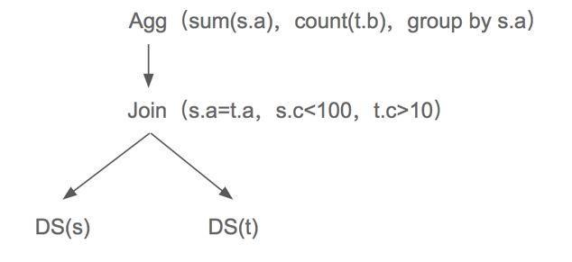
Then we will combine the following picture and code for a detailed introduction to explain how the baseLogicalPlan.findBestTask function work.
In the figure, the black font operator is a logical operator(e.g, Agg, Join and DS), the blue font is a physical operator(e.g, Stream Agg, Hash Join and Index Scan(a)...), and the yellow arrow is an operator for which the cost has been calculated. And the red dashed arrow is not in compliance with prop operator. The font on the arrow describes the property requirements for the lower operators(e.g, s.a means the the output of the lower operator needs to be ordered according to s.a).
Step1: ThegetTaskfunction corresponds to the yellow arrow in the figure, which means that the calculated part can be used directly without repeated calculations.Step2: Thep.self.exhaustPhysicalPlans(prop)function represents the process of logical operators generating physical operators. And it corresponds to the logical operator represented by the black font pointing to the physical operators represented by the blue font in the figure. For example, logical operatorAgggenerates physical operatorsStream AggandHash Agg. But some physical operators that do not satisfy the required property cannot be generated. For example, if the required property iss.alogical operatorDS, only physical operatorIndex Scan(a)can be generated, butTableScancannot be generated.Step3: After we generate all the possible physical plans, we should compare their costs and choose the lowest cost plan. For example, for the plan ofStream Agg -> Sort Merge Join -> Index Scan(a), its cost isCost(Stream Agg) + Cost(Sort Merge Join) + Cost(Index Scan(a)).
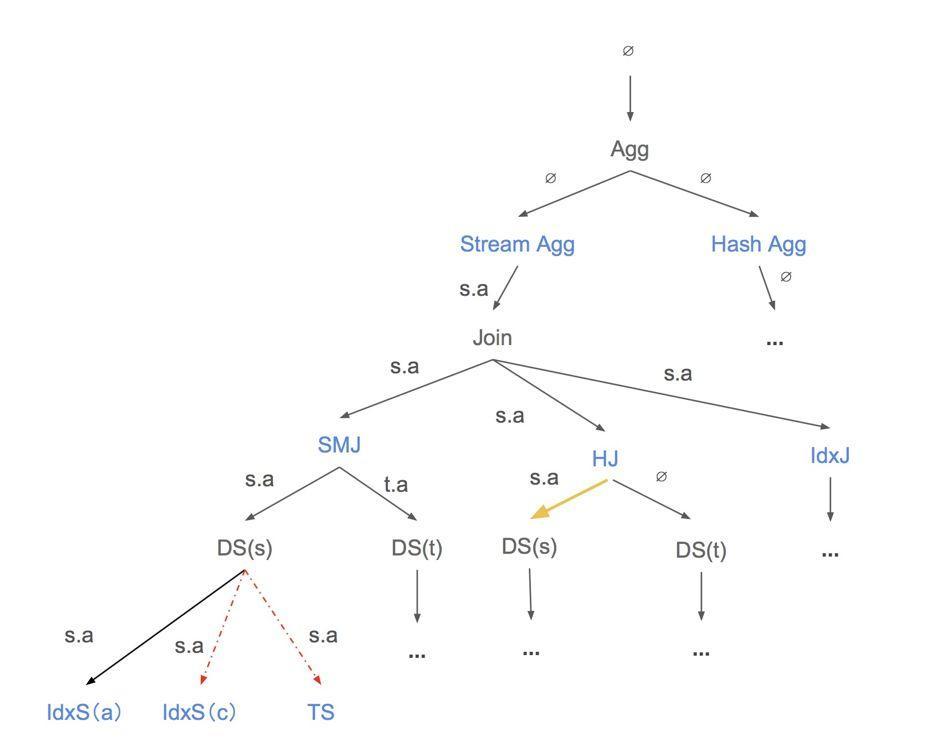
Exhaust Physical Plans
For each operator, the logic for exhausting physical plans are in exhaustPhysicalPlans(*property.PhysicalProperty) (physicalPlans []PhysicalPlan) method of the LogicalPlan interface. Their specific implementation is in the planner/core/exhaust_physical_plans.go file.
exhaustPhysicalPlans generates all possible plans that can match the required property. Different operators have different implementations. You can learn more about how different logical operators generate corresponding physical operators based on the required property by reading the code.
Enumerate Physical Plans For Task
Enumerate Physical Plans For Task will use the dynamic programming algorithm to select the lowest cost plan among all generated physical plans and it will return the task which encapsulates the selected physical plan. The task is a new version of physical plan. It stores cost information for a physical plan. You can see the interface definition of task in the planner/core/task.go file. A task may be copTask, rootTask, or a mppTask. copTask is a task that runs in a distributed kv store. rootTask is the task that runs in the TiDB compute layer. mppTask is a task that related to the mpp plan.
The introduction described in this section is based on the baseLogicalPlan.enumeratePhysicalPlans4Task function in the planner/core/find_best_task.go file. The simplified code is as follows:
func (p *baseLogicalPlan) enumeratePhysicalPlans4Task(physicalPlans []PhysicalPlan) task {
	bestTask = invalidTask

	for _, pp := range physicalPlans {
		for j, child := range p.children {
			childReqProps = pp.GetChildReqProps(j)
			// Get the best child tasks that can match the required property.
			childTasks[j] = child.findBestTask(childReqProps) // Step1
		}

		// Combine the best child tasks with parent physical plan.
		curTask = pp.attach2Task(childTasks...) // Step2

		// Get the most efficient one.
		if curTask.cost() < bestTask.cost() { // Step3
			bestTask = curTask
		}
	}
	return bestTask
}
The input of theenumeratePhysicalPlans4Task function is []PhysicalPlan, which represents all physical plans corresponding to logical plan p that meet the property requirements. And the output is the task which encapsulates the physical plan. This function can be divided into some parts.
-
For each physical plan, get the required property for their children first. And recursively call
findBestTaskto find the best child task that satisfies the required property. -
After we find the best children tasks, we should use the
pp.attach2Taskto combine them with the current physical operatorpp. Theattach2Task(...task) taskis the method ofPhysicalPlaninterface. It makes the current physical plan as the father of task's physical plan and updates the cost of current task. For each operator, you can see their special implementations in theplanner/core/task.gofile.In addition, the cost of one implementation is calculated as a sum of its resource consumptions including CPU, Memory, Network, IO, etc. For each kind of resource specifically, the consumption is measured based on a unit factor (e.g,
scanFactoris the unit factor for IO consumption, which means the cost of scanning 1 byte data onTiKVorTiFlash), and the estimated number of rows / bytes to be processed by this operator. Note that, these unit factors can be customized by setting system variables liketidb_opt_xxx_factorto fit clusters of different hardware configurations in thesessionctx/variable/session.gofile. -
Compare the current task to the best task and choose the most efficient one.
Summary
This chapter specifically introduces the Volcano Optimizer currently used by TiDB. We describe in detail how cost-based optimization selects a physical plan with the least cost based on statistics and cost models.
But we still have some problems that the current framework can not handle. For example:
- The operator push-down logic is too simple. Only one operator is allowed except
Selection, and it is difficult to deal with new push-down operators added in the future (such asProjection, etc.). - Poor scalability: it is difficult to expand to support other storage engines, and implement corresponding push-down operators, such as
TiFlash. - For optimization rules that may not always get better, we currently do not support the selection of rules through cost. The search space of the optimizer is restricted.
- ...
We want to solve these problems, so we are planning to develop a new optimizer framework the Cascades Planner. But it still works in progress. You can learn more by reading planner/cascades, planner/memo and planner/implementation under the planner module.
Plan Cache
Introduction
TiDB supports PlanCache for prepare and execute statements. By using PlanCache, TiDB can skip the optimization phase to gain some performance benefits.
There are several limitations to current PlanCache:
- Only support
prepareandexecutestatements, not support general queries; - Only session-level
PlanCacheis supported, cached plans cannot be reused across sessions; - Some complex plans cannot be cached, and you can see this document for more details;
Handling Prepare/Execute Statement
The process of handling a prepare statement is below:
- Parse the original SQL to an AST;
- Encapsulate the AST with some other necessary information(like
current-db,statement-text, ...) toCachedPrepareStmt; - Store the
CachedPrepareStmtinto this session'sPreparedStmtMap;
The process of handling an execute statement is below:
- Parse all parameters and store their values into this session's
PreparedParamMap; - Get the corresponding
CachedPrepareStmtfrom this session'sPreparedStmtMap; - Construct the plan-cache key with information in
CachedPrepareStmt; - Fetch a plan from the session's
PlanCacheby using this key, and:- if it succeeds, then
- check whether this plan is valid for current parameters, if it is, then
- rebuild the plan, and
- run the rebuilt plan;
- else, then
- optimize the AST in
CachedPrepareStmtwith current parameters to get a new plan, - store the new plan into current session's
PlanCache, and - run the new plan.
- optimize the AST in
- if it succeeds, then
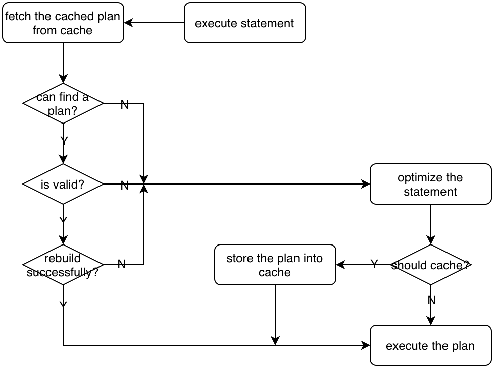
The main function of handling execute is common_plans.go:Execute.getPhysicalPlan().
Plan Rebuilding
A cached plan cannot be reused directly unless it is rebuilt. The main goal of rebuilding is to re-calculate the access range.
For example, if the query is select * from t where a<?, when you first execute it with 1, then a TableScan with range (-INF, 1) could be generated and cached, and then you later execute it with 2, the range has to be re-calculated to (-INF, 2) so that it can read correct data this time, and that is what plan rebuilding does.

The entry function of plan rebuilding is common_plans.go:Execute.RebuildPlan().
The Parameter Maker
Parameter Makers are used to propagate current parameter values to executors(operators).
For example, if the query is select * from t where a+?>1, then the filter a+?>1 will be converted to a Selection operator with an expression-tree a+?>1:
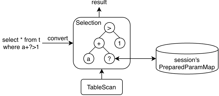
The parameter placeholder(?) is converted to a ParamMaker in Constant.
You can regard it as a special kind of pointer, and when the plan is processed and the parameter's value is needed, we can use it to get the corresponding value of this parameter.
type Constant struct {
    ...
    ParamMaker *ParamMaker
}

func (c *Constant) Eval(row) Datum {
    if c.ParamMaker != nil {return c.ParamMaker.GetUserVal()}
    ...
}

func (d *ParamMaker) GetUserVal() Datum {
    return d.ctx.GetSessionVars().PreparedParams[d.order]
}
SQL Plan Management
Execution
The executor package contains most of the codes related to execution. The input of the executor is a plan tree of the query returned from the planner, and the output of the executor is the result of the query. The entry function of execution module is executorBuild::build, the output result is fetched in clientConn::writeChunks.
Execution Framework
TiDB builds the computing engine based on the distributed storage provided by TiKV. The TiKV server implements a coprocessor framework to support distributed computing. The computing operations will be pushed to the TiKV coprocessor as far as possible to accelerate the computation speed. That is to say, a sub-plan of the SQL execution plan will be executed in parallel on different TiKV servers, and the result of each sub-plan will be collected to a TiDB server to compute for the final result.
The processing model of the execution plan tree is known as the Volcano iterator model. The essential of the Volcano model is abstracted to 3 interfaces: Open, Next, and Close. All operators offer the same interfaces and the implementation is opaque.
Open will be invoked in turn for each operator to init the needed resources before computing. Conversely, Close will release the resources. To obtain the query output, the final operator in the plan tree will keep invoking Next until no tuple is pulled from its child.
It's easy to understand how the Volcano model works for single-process execution. For parallelism issues, the Volcano introduces an operator called Exchange at any desired point in a plan tree. Further explanation about the parallelism-related issues would be introduced in the Parallel Execution Framework section.
Vectorized Execution
Vectorization uses the Volcano iteration model where each operator has a Next method that produces result tuples. However, each Next call fetches a block of tuples instead of just one tuple.
The main principle of vectorized execution is batched execution on a columnar data representation: every "work" primitive function that manipulates data does not work on a single data item, but on a vector (an array) of such data items that represents multiple tuples. The idea behind vectorized execution is to amortize the iterator call overhead by performing as much as possible inside the data manipulation methods. For example, this work can be to hash 1000s of values, compare 1000s of string pairs, update a 1000 aggregates, or fetch a 1000 values from 1000s of addresses.
Columnar Different from the row-oriented data representation, columnar format organize data by column rather by row. By storing data in columns rather than rows, the database can more precisely access the data it needs to answer a query rather than scanning and discarding unwanted data in rows. The memory columnar data representation in TiDB is defined as Chunk, which is inspired by Apache Arrow.
The detailed definition and usage of Chunk will be introduced in the Implementation of Vectorized Execution section.
Memory Management Mechanism
In TiDB, we set a memory usage quota for a query, and introduce two interfaces called Tracker and OOMAction for memory management.
The Tracker is used to track the memory usage of each element. The OOMAction is used to abstract the strategies to be used when the memory usage of a SQL exceeds the memory quota.
For example, we define the spill to disk strategy as SpillDiskAction. SpillDiskAction might be triggered by HashJoin or Sort when the memory quota is exceeded. If a query requires an order guarantee, and there is no index to guarantee the order, then the execution must sort the input before proceeding. If the input is small then the sort occurs in memory. We can split the input into multiple partitions and perform a merge sort on them. If the input is large, the SpillDiskAction will be triggered, an external sort algorithm is used. External sorting algorithms generally fall into two ways, sorting and merge. In the sorting phase, chunks of data small enough to fit in main memory are read, sorted, and written out to a temporary file. In the merge phase, the sorted subfiles are combined, and the final result will be outputted.
For more details, you can refers to the Memory Management Mechanism section.
Typical Operators
TiDB implements multiple algorithms for the Join, Aggregation, Sort operators, and so on. We'll take some of them for detailed introduction. If you are interested, you can refer to the Implementation of Typical Operators section.
Parallel Execution Framework
In order to make full use of the multi-core ability of modern hardware, most popular DBMS have implemented the ability of parallel execution SQL execution engine.
There are three common parallel implementations: Intra operator parallelism, Exchange operator, and Morsel-Driven parallelism. And TiDB adopts the first approach.
TiDB Implementation
In intra-operator parallelism, multiple goroutines will be created inside the operator for parallel processing. The creation, termination and synchronization of the goroutines are handled by the operator itself.
Most operators will create multiple goroutines in Open() or the first call of Next(). And they will wait on channels for input Chunk. Also, a special channel is responsible for notifying whether to stop the computation. And WaitGroup can be used to wait for the termination of all goroutines. This usually happens when Close() is called.
Taking HashJoin as an example, all workers will be started at the first call of Next(), including:
- buildSideFetcher: Will call
buildSideExec.Next()to fetch input Chunk. - builderWorker: Receive data from the buildSideFetcher and build the HashTable.
- probeSideFetcher: Wait for the end of building of the HashTable and call
probeSideExec.Next()to fetch input Chunk. - probeWorker: Receive data from the probeSideFetcher and then probe the HashTable.
When the main goroutine calls HashJoinExec.Next(), it will read data from the result channel and send an empty Chunk to the resource channel. When HashJoinExec.Close() is called, a special channel will be closed and all workers waiting on the channel will exit.
The parallel implementations of operators are various. For example, HashAgg is divided into two stages. Each stage will start multiple goroutines (partialWorkers and finalWorkers).
It is worth noting that we still use the traditional Volcano-model, the Next() is only called by a single thread. The parallelism only occurs in the internal processing of the operator.
The degree of parallelism (DOP) can be controlled by the session variable. For example, tidb_executor_concurrency is 5 by default. It means HashJoin will create five goroutines to probe HashTable. You can also control the parallelism of a specific operator by changing the session variable, such as tidb_hash_join_concurrency.
At present, most important operators have implemented intra-operator parallelism:
- Join: HashJoin, IndexJoin, IndexHashJoin, IndexMergeJoin
- Apply: ParallelApply
- Aggregation: HashAgg
- Other: Union, Projection
- Reader: TableReader, IndexReader
Other operators are still single threaded: TopN, Limit, Sort, MergeJoin, StreamAgg, Selection, WindowFunc. But some of them (TopN, Limit, StreamAgg, Selection) can be pushed down to TiKV.
Other Parallelism Implementation
Intra operator parallelism is the most intuitive way to implement parallelism, but its implementation is complex, because every operator needs to implement parallelism independently. What's worse, too many threads will increase the scheduling overhead. Although, the use of goroutines can alleviate this problem.
A more traditional way to implement parallelism is to use the exchange operator. By encapsulating the parallel logic into the exchange operator, all other operators only need to consider the single thread implementation.
The exchange operator is responsible for data exchange between different threads. The internal implementation of exchange is divided into two parts: sender and receiver. And data is transferred from sender to receiver in different ways, such as hash partition, random distribution or sort merge.
There are usually two ways to control DOP:
- Users can use hints to specify DOP explicitly.
- The optimizer can choose DOP according to the table size of the scan operation automatically.
This approach requires the optimizer to generate parallel plans. Generally, plan generation is divided into two stages. The first stage generates serial plans, and the second stage generates its corresponding parallel plans. The second stage is mainly responsible for inserting the exchange operator into the plan tree at the appropriate position. Both heuristic rules and cost model can be used to get the optimal parallel plan.
Currently, TiDB has a simplified implementation of exchange operator: Shuffle Operator. It can make MergeJoin, StreamAgg and WindowFunc run in parallel. And you can enable MergeJoin to be parallel by setting tidb_merge_join_concurrency be greater than 1.
For Morsel-Driven, it implements parallelism by dividing data into fixed size blocks (Morsel: usually 100000 rows). And a customized scheduler will be responsible for task scheduling to achieve better load balancing. And TiDB doesn't use this approach for now.
Implementation of Vectorized Execution
This section introduces the implementation details of the TiDB vectorized execution model.
Understanding Vectorized Execution
Vectorized execution, also known as batch processing, is a method of processing data in batches, rather than row by row. Traditional row-based processing handles one row at a time, which can lead to significant overhead and reduced efficiency, especially when dealing with large datasets. Vectorized execution, on the other hand, processes data in chunks or vectors, allowing for better utilization of CPU and memory resources.
Key Benefits of Vectorized Execution
- Improved CPU Utilization: Processing data in batches minimizes the overhead associated with instruction fetching and decoding, leading to better CPU utilization and improved performance.
- Reduced Memory Access: Data processed in vectors is more likely to be present in the CPU cache, reducing the need for memory access, which is often a performance bottleneck.
- Reduced Branching: Traditional row-based processing often involves conditional statements and branching, which can hinder performance. Vectorized execution minimizes branching, leading to more predictable and faster execution.
Implementing Vectorized Execution in TiDB
TiDB leverages a memory layout similar to Apache Arrow to enable the execution of a batch of data at a time. This approach allows for efficient data processing, reducing overhead and improving performance.
Columnar Memory Layout Implementation in TiDB
In TiDB, the columnar memory layout is defined as a Column, and a batch of these Columns is referred to as a Chunk. The implementation of Column draws inspiration from Apache Arrow, ensuring efficient data processing. Depending on the data type they store, TiDB employs two types of Columns:
- Column with Fixed Length: These Columns store data of a fixed length, such as Double, Bigint, Decimal, and similar data types. This structure is optimized for predictable and consistent data sizes, facilitating efficient processing.
- Column with Variable Length: These Columns accommodate variable-length data types, including Char, Varchar, and others. Variable-length data types can hold a range of character lengths, and the Column structure adapts to handle such variability. In TiDB, the Column and Chunk types are defined as follows:
type Column struct {
    length     int      // the number of elements in the column
    nullBitmap []byte   // bitmap indicating null values
    offsets    []int64  // used for varLen column; row i starts from data[offsets[i]]
    data       []byte   // the actual data
    elemBuf    []byte   // used to indicate the byte length of each element for fixed-length objects
    // ... (additional fields)
}

type Chunk struct {
    columns  []*Column
    sel      []int      // sel indicates which rows are selected. If it is nil, all rows are selected.
    capacity int        // capacity indicates the maximum number of rows this chunk can hold.
    // ... (additional fields)
}
Column and Chunk Data Manipulation
TiDB supports various data manipulation operations on Column and Chunk:
Appending a Fixed-Length Non-NULL Value to a Column:
- To append an element, a specific
appendmethod tailored to the data type is called (e.g., AppendInt64). - The data to be appended is shallow copied to the
elemBufusing anunsafe.Pointer. - The data in
elemBufis then appended to thedata. - A
1is appended to thenullBitmap.
Appending a Non-Fixed-Length Non-NULL Value to a Column:
- To append a variable-length data value, such as a string, it is directly appended to the
data. - A
1is appended to thenullBitmap. - The starting point of the newly appended data in the
datais recorded in theoffsets.
Appending a NULL Value to a Column:
- To append a NULL value, the AppendNull function is used.
- A
0is appended to thenullBitmap. - If it's a fixed-length column, a placeholder data of the same size as
elemBufis appended to thedata. - If it's a variable-length column, no data is appended to the
data, but the starting point of the next element is recorded in theoffsets.
Reading a Value from a Column:
- Values in a
Columncan be read using functions like GetInt64(rowIdx) and GetString(rowIdx). The reading principle can be deduced from the previously described appending mechanism. Here, we retrieve the specified element in theColumnbased on the rowID. The details of reading from aColumnare consistent with the principles discussed for appending.
Reading a Row from a Chunk:
- Within a
Chunk, the concept of a Row is logical. The data for a row is stored across differentColumnsin theChunk. The data for the same row in various columns is not necessarily stored consecutively in memory. When obtaining aRowobject, there is no need to perform data copying, as the data for the same row is already stored in the correspondingColumns. - The concept of a
Rowis useful because, during the operation of operators, data is often accessed and processed on a per-row basis. For example, operations like aggregation, sorting, and similar tasks work with data at the row level. - You can retrieve a row from a
Chunkusing the GetRow(rowIdx) function. Once you have aRowobject, you can further access the data in specific columns within that row using functions like Row::GetInt64(colIdx), which allows you to retrieve the data corresponding to the specified column index for that row.
Examples
How expression is evaluated
In this section, we’ll use the TiDB expression colA * 0.8 + colB to demonstrate how expression evaluation works using vectorized execution and to highlight the performance gap between row-based execution and vectorized execution.
Expression Tree Representation
The TiDB expression colA * 0.8 + colB is parsed into an expression evaluation tree, where each non-leaf node represents an arithmetic operator, and the leaf nodes represent the data source. Each non-leaf node can be either a constant (like 0.8) or a field (like colA) in the table. The parent-child relationship between nodes indicates a computationally dependent relationship: the evaluation result of the child node is the input data for the parent node.
                             ┌─┐
                         ┌───┤+├───┐
                         │   └─┘   │
                        ┌┴┐       ┌┴┐
  colA*0.8+colB───►  ┌──┤*├───┐   │B│
                     │  └─┘   │   └─┘
                    ┌┴┐     ┌─┴─┐
                    │A│     │0.8│
                    └─┘     └───┘
Non-Vectorized Execution
In a non-vectorized execution model, the computing logic of each node can be abstracted using the following evaluation interface:
type Node interface {
    evalReal(row Row) (val float64, isNull bool)
}
Taking *, 0.8, and col nodes as examples, all three nodes implement the interface above. Their pseudocode is as follows:
func (node *multiplyRealNode) evalReal(row Row) (float64, bool) {
    v1, null1 := node.leftChild.evalReal(row)
    v2, null2 := node.rightChild.evalReal(row)
    return v1 * v2, null1 || null2
}

func (node *constantNode) evalReal(row Row) (float64, bool) {
    return node.someConstantValue, node.isNull  // 0.8 in this case
}

func (node *columnNode) evalReal(row Row) (float64, bool) {
    return row.GetReal(node.colIdx)
}
In non-vectorized execution, the expression is iterated over rows. Every time this function performs a multiplication, only a few instructions are actually involved in the "real" multiplication compared to the number of assembly instructions required to perform the function.
Vectorized Execution
In vectorized execution, the interface to evaluate an expression in a batch manner in TiDB looks like this:
type VecNode interface {
  vecEvalReal(input *Chunk, result *Column)
}
Taking multiplyRealNode as an example:
func (node *multiplyRealNode) vecEvalReal(input *Chunk, result *Column) {
  buf := pool.AllocColumnBuffer(TypeReal, input.NumRows())
  defer pool.ReleaseColumnBuffer(buf)
  node.leftChild.vecEvalReal(input, result)
  node.rightChild.vecEvalReal(input, buf)

  f64s1 := result.Float64s()
  f64s2 := buf.Float64s()
  result.MergeNulls(buf)
  for i := range i64s1 {
     if result.IsNull(i) {
        continue
     }
     i64s1[i] *= i64s2[i]
  }
}
This implementation reduces the interpretation overhead by batch processing, which is more beneficial for modern CPUs:
- A vector of data is sequentially accessed. This reduces CPU cache misses.
- Most of the computational work is within a simple loop. This facilitates CPU branch prediction and instruction pipelining.
We use the same dataset (1024 rows formed by two columns of floating-point numbers) to compute colA * 0.8 + colB in two ways: row-based execution and vectorized execution. The results are as follows:
BenchmarkVec-12           152166              7056 ns/op               0 B/op          0 allocs/op
BenchmarkRow-12            28944             38461 ns/op               0 B/op          0 allocs/op
The results above show vectorized execution is four times faster than row-based execution. For more details about the vectorized expression evaluation, you can refer to this link.
How operators are evaluated
In this section, we'll dive deeper into the evaluation of operators, focusing on HashJoin as an example.
HashJoin in vectorized execution consists of the following steps:
Hashing Phase
Let's consider the table used for constructing the hash table as 't'. The data from table 't' is read into Chunk in batches. First, the data in the Chunk is filtered by columns based on the predicates on table 't'. The filtered results for these columns are then combined into a selected array. In the selected array, true values indicate valid rows. The relevant code is available in the VectorizedFilter section.
Subsequently, the hash values for the remaining valid data in the Chunk are calculated column-wise. If multiple columns are used in the hash, their values are concatenated to form the final hash key for a row. Further details can be found in the HashChunkSelected code section.
Finally, the selected array is used for filtering. The hash key for valid rows, along with their corresponding row pointers, is used to construct the hash table.
Probe Phase
The probe phase in HashJoin mirrors the build phase. Initially, data from the probe table is read into Chunk in batches. Predicates are applied to filter the Chunk by columns, and a selected array is generated to mark valid rows. The hash keys are then calculated for each of the valid rows.
For the valid rows in the Chunk, the calculated hash value is employed to probe the hash table constructed during the build phase. This lookup aims to identify matching rows in the hash table using the hash values. The implementation can be explored in join2Chunk.
Matching and Output
Upon discovering matching rows in the hash table, the outcomes are output as joined rows and saved in a new Chunk. For deeper insights, see the code in joinMatchedProbeSideRow2Chunk.
Vectorized computation in HashJoin offers considerable advantages over row-based computation, primarily concerning performance. By allowing for batch processing of data, vectorized computation minimizes instruction fetch and decode overhead, enhancing CPU utilization, trimming memory access, reducing conditional branches, and augmenting parallelism. These benefits render vectorized HashJoin exceptionally efficient and performant when processing large datasets.
Conclusion
In conclusion, TiDB's adept data processing, drawing inspiration from the Apache Arrow memory layout with its columns and chunks, emerges as an invaluable asset for contemporary data professionals. With its vectorized execution, TiDB heightens CPU utilization, curtails memory access overhead, and curbs branching, culminating in substantially accelerated and more streamlined query performance.
Memory Management Mechanism
TiDB's memory management basically consists of a memory usage quota settings for each query, and two interfaces, called Tracker and OOMAction.
Tracker
Tracker tracks the memory usage of each element with a tree structure.
Genral use cases:
                                               /--- Tracker(Component in Executor, e.g. list/rowContainer/worker)
                                               |           ...
                    /--- Tracker(Executor1) ---+--- Tracker(Component)
                    |
Tracker(Session) ---+--- Tracker(Executor2)
      |             |         ...
      |             \--- Tracker(Executor3)
 OOM-Action1
      |
      |
 OOM-Action2
     ...
When a component allocates some memory, it will call the function Tracker.Consume(bytes) to tell the Tracker how much memory it uses. Tracker.Comsume will traverse all its ancestor nodes, accumulate memory usage and trigger OOM-Action when exceeded.
OOM-Action
OOM-Action is a series of actions grouped in a linked list to reduce memory usage. Each node on the linked list abstracts a strategy to be used when the memory usage of a SQL exceeds the memory quota. For example, we define the spill to disk strategy as SpillDiskAction, rate limit strategy as rateLimitAction and cancel strategy as PanicOnExceed.
Rate Limit
TiDB supports dynamic memory control for the operator that reads data. By default, this operator uses the maximum number of threads that tidb_disql_scan_concurrency allows to read data. When the memory usage of a single SQL execution exceeds tidb_mem_quota_query each time, the operator that reads data stops one thread.
We use rateLimitAction to dynamically control the data reading speed of TableReader.
Spill Disk
TiDB supports disk spill for execution operators. When the memory usage of a SQL execution exceeds the memory quota, tidb-server can spill the intermediate data of execution operators to the disk to relieve memory pressure. Operators supporting disk spill include Sort, MergeJoin, HashJoin, and HashAgg.
SpillDiskAction
We use SpillDiskAction to control the spill disk of HashJoin and MergeJoin. The data will be placed in Chunk unit when spilling. We can get any data in Chunk through random I/O.
SortAndSpillDiskAction
We use SortAndSpillDiskAction to control the spill disk of Sort.
If the input of SortExec is small, then it sorts in memory. If the input is large, the SortAndSpillDiskAction will be triggered, and an external sort algorithm will be used. We can split the input into multiple partitions and perform a merge sort on them.
External sorting algorithms generally have two stages, sort and merge. In the sort stage, chunks of data small enough to fit in main memory are read, sorted, and written out to a temporary file. In the merge stage, the sorted subfiles are combined, and the final result will be outputted.
AggSpillDiskAction
We use AggSpillDiskAction to control the spill disk of HashAgg. When AggSpillDiskAction is triggered, it will switch HashAgg executor to spill-mode, and the memory usage of HashAgg won't grow.
We use the following algorithm to control the memory increasing:
- When the memory usage is higher than the
mem-quota-query, switch the HashAgg executor to spill-mode. - When HashAgg is in spill-mode, keep the tuple in the hash map no longer growing. a. If the processing key exists in the Map, aggregate the result. b. If the processing key doesn't exist in the Map, spill the data to disk.
- After all data have been processed, output the aggregate result in the map, clear the map. Then read the spilling data from disk, repeat the Step1-Step3 until all data gets aggregated.
As we can see, unlike other spilling implementations, AggSpillDiskAction does not make the memory drop immediately, but keeps the memory no longer growing.
Log/Cancel
When the above methods cannot control the memory within the threshold, we will try to use PanicOnExceed to cancel the SQL or use LogOnExceed to log the SQL info.
Implementation of Typical Operators
This section introduces the implementation details of three typical TiDB operators: Sort, HashAgg, and HashJoin.
Firstly, every operator should implement three basic interfaces of Executor:
- Open - Initializes the operator, sets up the memory tracker/disk tracker, and other meta-info for the current operator.
- Next - Each call to
Nextreturns a chunk of data. Returning an empty chunk indicates that the execution is complete for the current executor. Note thatNextis not thread-safe. It's by design thatNextis not called concurrently for all operators. - Close - Responsible for releasing all resources held by the executor.
Sort
The Sort operator is used to arrange the result set of a query in a specific order. In TiDB, the operator implementing sort is SortExec. The fundamental concept behind SortExec is to read all the data from its child executor and then sort the entire data set.
In Next, it invokes fetchRowChunks to read all the data from its child executor. fetchRowChunks aims to store all the data in one SortedRowContainer. The memory usage grows as the input data volume increases. To manage the memory usage, SortExec has spill-to-disk support. The details of this spilling are encapsulated within SortedRowContainer. Every time the insertion of a chunk into the current SortedRowContainer returns ErrCannotAddBecauseSorted, it indicates that the current SortedRowContainer has been spilled. SortExec will then create a new SortedRowContainer and insert the chunk into this new container. Once there's no data coming from its child executor, SortExec will sort the current SortedRowContainer.
After fetchRowChunks completes, Next starts producing sorted results. Depending on whether a spill to disk was initiated, there are two methods to produce the final sorted outcomes:
- Spill not initiated: In this straightforward scenario, if there's no spill, since the entire
SortedRowContainergets sorted at the end offetchRowChunks, duringNext, it simply invokesGetSortedRowAndAlwaysAppendToChunkto fetch the sorted data fromSortedRowContainer. - Spill initiated: When a spill occurs, each spilling round produces an independent
SortedRowContainer, stored inpartitionList. InNext, an external multi-way merge sort merges all partially sorted data streams into one final sorted data stream.
HashAgg
The HashAgg operator uses a hash table to perform grouping and aggregation. In TiDB, the operator implementing hash aggregation is HashAggExec.
HashAgg has two execution modes: parallel and non-parallel execution. During the build stage, the planner is responsible for deciding the execution mode for a HashAgg. A HashAgg will operate in non-parallel execution mode if one of the following conditions is true:
- The aggregation function contains
distinct. - The aggregation function (
GROUP_CONCAT) containsorder by. - The user explicitly sets both
hashAggPartialConcurrencyandhashAggFinalConcurrencyto 1.
Non-parallel Execution
Non-parallel execution mode performs aggregation in a single thread. unparallelExec is the core function for non-parallel execution. In unparallelExec, it first reads all the data from its child executor, then aggregates the data using execute. After execute completes, unparallelExec starts to generate results by traversing all the group-by keys, generating one row for each key by calling AppendFinalResult2Chunk for each aggregation function.
Parallel Execution
Parallel execution mode performs aggregation using multiple threads, dividing the aggregation into two stages:
- Partial stage: each thread aggregates a portion of the input data into partial results.
- Final stage: each thread aggregates the partial results into final results.
The flow of parallel execution is illustrated in the following graph:
                            +-------------+
                            | Main Thread |
                            +------+------+
                                   ^
                                   |
                                   +
                              +-+-            +-+
                              | |    ......   | |  finalOutputCh
                              +++-            +-+
                               ^
                               |
                               +---------------+
                               |               |
                 +--------------+             +--------------+
                 | final worker |     ......  | final worker |
                 +------------+-+             +-+------------+
                              ^                 ^
                              |                 |
                             +-+  +-+  ......  +-+
                             | |  | |          | |
                             ...  ...          ...    partialOutputChs
                             | |  | |          | |
                             +++  +++          +++
                              ^    ^            ^
          +-+                 |    |            |
          | |        +--------o----+            |
 inputCh  +-+        |        +-----------------+---+
          | |        |                              |
          ...    +---+------------+            +----+-----------+
          | |    | partial worker |   ......   | partial worker |
          +++    +--------------+-+            +-+--------------+
           |                     ^                ^
           |                     |                |
      +----v---------+          +++ +-+          +++
      | data fetcher | +------> | | | |  ......  | |   partialInputChs
      +--------------+          +-+ +-+          +-+
There are three types of threads that read data and execute the aggregation:
fetchChildData: This thread's concurrency level is set to 1. It reads data from the child executor and places it intoinputCh, serving as the input for each partial worker.HashAggPartialWorker: The concurrency ofHashAggPartialWorkeris determined byhashAggPartialConcurrency. This worker reads the input data, executes partial aggregation on the data, produces partial results, and sends them to the final worker.HashAggFinalWorker: The concurrency ofHashAggFinalWorkeris set byhashAggFinalConcurrency. This worker reads partial results, produces final results, and sends them tofinalOutputCh.
Similar to Sort, HashAgg is also a memory-intensive operator. When HashAgg runs in non-parallel execution mode, it supports spill-to-disk functionality (spill-to-disk in parallel execution mode is currently under development). Unlike Sort, which spills all data to disk, the HashAgg approach is different. In the current implementation, once a HashAgg is flagged for spilling, for all subsequent inputs, if the group-by key of a row already exists in the current hash map, the row will be inserted into the hash map. If not, the row gets spilled to disk. Detailed workings of the HashAgg spill can be explored here.
HashJoin
The HashJoin operator uses a hash table to perform the join operation. In TiDB, the operator that implements hash join is HashJoinExec.
HashJoin constructs the results in two distinct stages:
- Fetch data from the build side child and build a hash table.
- Fetch data from the probe side child and probe the hash table using multiple join workers.
Build stage
The fetchAndBuildHashTable function orchestrates the build stage. Two threads are engaged in this work:
- fetchBuildSideRows reads data from the build side child and funnels it into the
buildSideResultCh. - buildHashTableForList retrieves input data from
buildSideResultChand subsequently constructs the hash table based on this input.
Detailed mechanics of building the hash table are encapsulated within the hashRowContainer. It's worth noting that, as of now, TiDB does not support the parallel building of hash tables.
Probe stage
The fetchAndProbeHashTable function executes the probe stage. This stage engages two types of threads:
fetchProbeSideChunksoperates with a concurrency of 1. It reads data from the probe child and dispatches them to various probe workers.probeWorkerinstances read data fromfetchProbeSideChunksand probe concurrently. The concurrency level is determined byExecutorConcurrency.
Each probeWorker contains a joiner, a core data structure implementing various join semantics. Every type of join in TiDB has its specialized joiner. The currently supported joiners include:
innerJoiner- For inner joinleftOuterJoiner- For left outer joinrightOuterJoiner- For right outer joinsemiJoiner- For semi joinantiSemiJoiner- For anti semi joinantiLeftOuterSemiJoiner- For anti left outer semi joinleftOuterSemiJoiner- For left outer semi joinnullAwareAntiSemiJoiner- For null aware anti semi joinnullAwareAntiLeftOuterSemiJoiner- For null aware anti left outer semi join
The joiner offers three foundational interfaces:
tryToMatchInners- For each row from the probe side, it attempts to match the rows from the build side. Returns true if a match occurs and setsisNullfor the special join types:AntiSemiJoin,LeftOuterSemiJoin, andAntiLeftOuterSemiJoin.tryToMatchOuters- Exclusive to outer join scenarios where the outer side acts as the build hash table. For each row from the probe (inner) side, it attempts to match the rows from the build (outer) side.onMissMatch- Used in semi join scenarios to manage cases where no rows from the build side match the probe row.
During the probeWorker operation, it reads data from the probe side. For every probe row, it attempts to match against the hash table and saves the result into a result chunk. Most of these operations utilize the join2Chunk function for probing. However, for outer joins that use the outer side as the build side, the function join2ChunkForOuterHashJoin is called upon.
Within join2Chunk/join2ChunkForOuterHashJoin, the probe work consists of three steps for each probe row:
- Quick tests are conducted before accessing the hash table to determine if a probe row won't find a match. For instance, in an inner join, if the join key contains null, the probe can bypass the hash table probing since null will never match any value. For rows that are non-matching, the
onMissMatchfunction is invoked. - The hash table is looked up to identify potential matching rows.
- In the absence of potential matching rows, the
onMissMatchfunction is invoked. Otherwise, thetryToMatchfunction is executed.
Transaction
The transaction engine in TiDB is responsible to provide ACID guarantees for all the read and write requests. It consists of the client/coordinator part in the TiDB repository and the server/participant part in the TiKV repository.
This document is mainly about the TiDB part.
The Architecture
In TiDB the transaction write flow is like this:
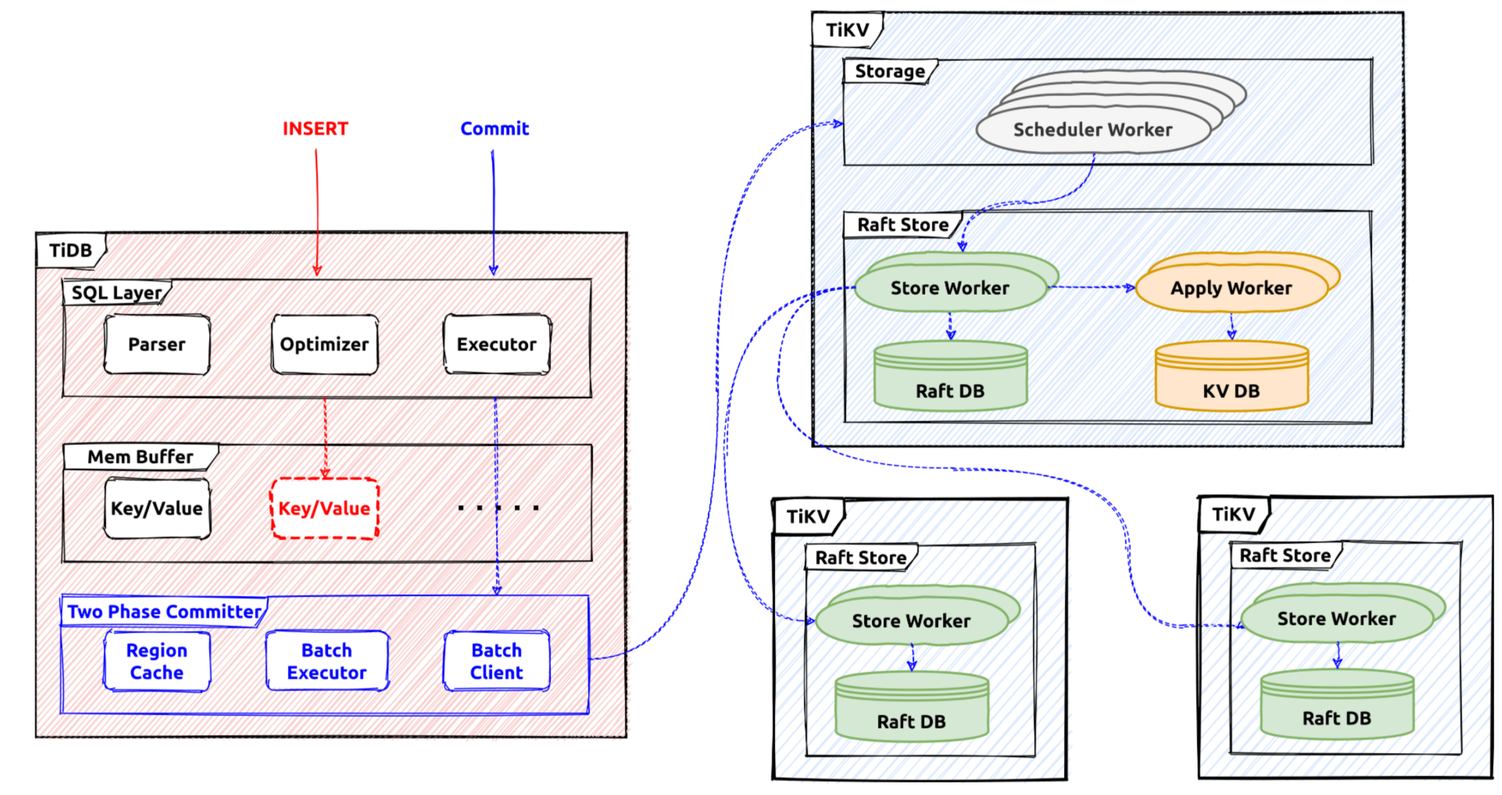
After the transaction starts in a session, all the reads and writes will use a snapshot to fetch data, and the written content will be buffered in the memory of the transaction. When the commit statement is received from the client, the Percolator protocol will be used to commit these changes to the storage system.
The Interface
In TiDB, the Transaction interface defines the commonly used transaction operations.
type Transaction interface {
	// Commit commits the transaction operations to KV store.
	Commit(context.Context) error
	// Rollback undoes the transaction operations to KV store.
	Rollback() error
	// LockKeys tries to lock the entries with the keys in KV store.
	// Will block until all keys are locked successfully or an error occurs.
	LockKeys(ctx context.Context, lockCtx *LockCtx, keys ...Key) error
	// SetOption sets an option with a value, when val is nil, uses the default
	// value of this option.
	SetOption(opt int, val interface{})
	// GetOption returns the option
	GetOption(opt int) interface{}
	...
	// StartTS returns the transaction start timestamp.
	StartTS() uint64
	// Valid returns if the transaction is valid.
	// A transaction become invalid after commit or rollback.
	Valid() bool
	// GetMemBuffer return the MemBuffer binding to this transaction.
	GetMemBuffer() MemBuffer
	// GetSnapshot returns the Snapshot binding to this transaction.
	GetSnapshot() Snapshot
}
These are common interfaces the transaction will provide.
For example, Commit will be used to commit the current ongoing transaction. The transaction is considered ongoing before the Commit operation is triggered. The two-phase commit processing will be used to commit a transaction and it will finally become committed or aborted.
LazyTxn is a wrapper of the transaction implementations, when the SQL statements are executed using a standalone session context, LazyTxn will be used to do things like:
- Return the memory buffer for write.
- Set specific operations or flags for the current transaction.
- Return the snapshot of this transaction.
- Commit the current transaction.
- Lock specific keys.
The Statement Execution
Usually, the first thing that will be done executing a statement is to activate the related transaction
By default, TiDB provides the snapshot isolation level. Thus, in each new transaction, a new global strong snapshot will be fetched first, before executing statements.
In TiDB, the snapshot is represented by a global TSO which is fetched from the PD server, and it acts as the unique identifier for this transaction. After this operation, a transaction is regarded as activated.
For the read SQL statements, the snapshot will be used to provide a global strong consistent snapshot, all the reads will check data visibility using this snapshot. Most executors will set the timestamp doing the build, and the transaction could be activated by the building process. Some commonly used snapshot APIs are as below:
// BatchGet gets all the keys' value from kv-server and returns a map contains key/value pairs.
// The map will not contain nonexistent keys.
func (s *tikvSnapshot) BatchGet(ctx context.Context, keys []kv.Key) (map[string][]byte, error) {
	data, err := s.KVSnapshot.BatchGet(ctx, toTiKVKeys(keys))
	return data, extractKeyErr(err)
}

// Get gets the value for key k from snapshot.
func (s *tikvSnapshot) Get(ctx context.Context, k kv.Key) ([]byte, error) {
	data, err := s.KVSnapshot.Get(ctx, k)
	return data, extractKeyErr(err)
}
For the write SQL statements, they will write data into the transaction memory buffer temporarily until the commit operation is triggered. There are 3 main interfaces which will write query data into the memory buffer. Here is the table API:
// Table is used to retrieve and modify rows in table.
type Table interface {
	// AddRecord inserts a row which should contain only public columns
	AddRecord(ctx sessionctx.Context, r []types.Datum, opts ...AddRecordOption) (recordID kv.Handle, err error)

	// UpdateRecord updates a row which should contain only writable columns.
	UpdateRecord(ctx context.Context, sctx sessionctx.Context, h kv.Handle, currData, newData []types.Datum, touched []bool) error

	// RemoveRecord removes a row in the table.
	RemoveRecord(ctx sessionctx.Context, h kv.Handle, r []types.Datum) error
}
Every statement will use a staging buffer during its execution. If it's successful, the staging content will be merged into the transaction memory buffer.
For example, AddRecord will try to write a row into the current statement staging buffer, and the RemoveRecord will try to remove a row from the staging statement buffer. The existing transaction memory buffer will not be affected if the statement has failed.
The memory buffer implementation is wrapped in memBuffer. The internal implementation is MemDB struct.
The memory buffer is an ordered map and it provides the staging and discard utilities. For example, the memory content generated by a statement will be discarded if its execution has failed.
The Two-phase Commit
After the statement execution phase, the commit statement will trigger the commit execution for the current transaction. In TiDB, the Percolator protocol is used as the distributed transaction protocol, it's a two-phase protocol.
In the first stage, the transaction coordinator (TiDB server) will try to prewrite all the related keys. If all of them are successful, the transaction coordinator will then commit the primary key. After that the transaction is considered committed successfully, and a success message will be responded to the client. All the other keys will be committed asynchronously.
All the changes in the transaction memory buffer will be converted into mutations which will be used by the two-phase committer. These mutations will be grouped by their region locations, and prewrite requests will be sent to their region leaders.
If all the prewrite requests are processed successfully, the commit request for the primary key will be sent to TiKV first. If the primary key commit is successful, the transaction is considered committed and will respond to the client with successful results.
Recommended Reading
Transaction on TiKV
The previous section introduces the architecture of the transaction engine and several implementation details in TiDB part. This document is mainly about the TiKV part.
As described in the previous section, the distributed transaction coordinator is tidb-server which receives and processes COMMIT query, and the transaction participants involved are tikv-servers.
Transactional Protocol
The RPC interfaces in TiDB are defined in a protobuf file, based on the Percolator model.
These interfaces will be used by the transaction coordinator to drive the whole commit process. For example Prewrite will be used to write the lock record in TiKV:
message PrewriteRequest {
    Context context = 1;
    // The data to be written to the database.
    repeated Mutation mutations = 2;
    // The client picks one key to be primary (unrelated to the primary key concept in SQL). This
    // key's lock is the source of truth for the state of a transaction. All other locks due to a
    // transaction will point to the primary lock.
    bytes primary_lock = 3;
    // Identifies the transaction being written.
    uint64 start_version = 4;
    uint64 lock_ttl = 5;
    // TiKV can skip some checks, used for speeding up data migration.
    bool skip_constraint_check = 6;
    // For pessimistic transaction, some mutations don't need to be locked, for example, non-unique index key.
    repeated bool is_pessimistic_lock = 7;
    // How many keys this transaction involves in this region.
    uint64 txn_size = 8;
    // For pessimistic transactions only; used to check if a conflict lock is already committed.
    uint64 for_update_ts = 9;
    // If min_commit_ts > 0, this is a large transaction request, the final commit_ts
    // will be inferred from `min_commit_ts`.
    uint64 min_commit_ts = 10;
    // When async commit is enabled, `secondaries` should be set as the key list of all secondary
    // locks if the request prewrites the primary lock.
    bool use_async_commit = 11;
    repeated bytes secondaries = 12;
    // When the transaction involves only one region, it's possible to commit the transaction
    // directly with 1PC protocol.
    bool try_one_pc = 13;
    // The max commit ts is reserved for limiting the commit ts of 1PC or async commit, which can be used to avoid
    // inconsistency with schema change.
    uint64 max_commit_ts = 14;
}
mutationsare changes made by the transaction.start_versionis the transaction identifier fetched from PD.for_update_tsis used by the pessimistic transactions.try_one_pcfield is used if the transaction is committed usingone-phaseprotocol.use_async_commitandsecondarieswill be used if the transaction is committed in theasync-commitmode.
Besides prewrite request, there are some other important request types:
pessimistic_lockrequest is used to lock a key. Note pessimistic locking happens in the transaction execution phase, for example aselect for updatestatement will need to pessimistically lock the corresponding rows.commitrequest is used to commit a key. After commit the write content is visible to other read or write transactions.check_txn_statusrequest will be used to check the status of a given transaction, so that it could be decided how to process the conflicts.resolverequest will be used to help doing the transaction crash recovery.check_secondary_locksrequest is a special API, it will be used if the commit mode of the transaction isasync-commit.
Transaction Scheduler
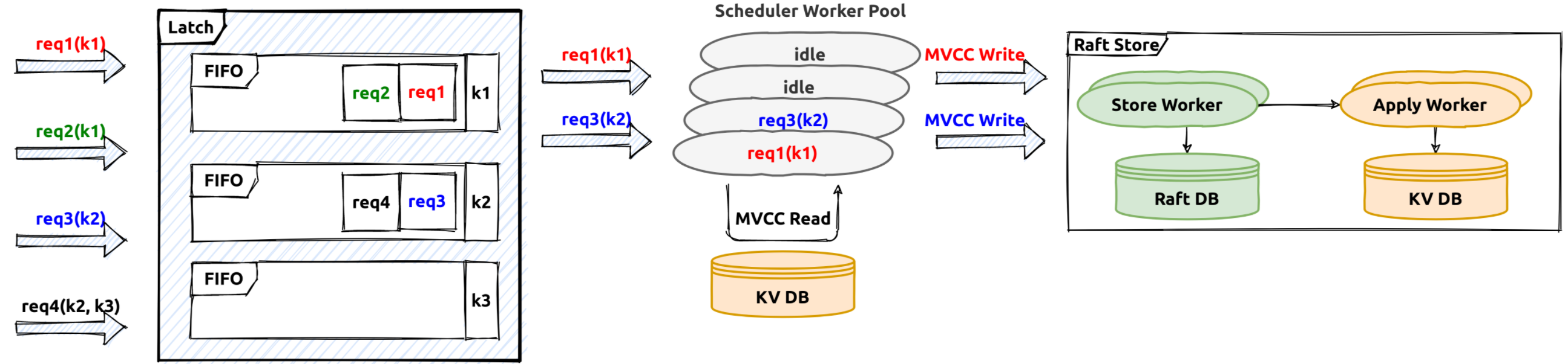
The receiving input transaction requests will be translated into transaction commands. Then the transaction scheduler will handle these transaction commands, it will first try to fetch the needed key latches (latch is used to sequence all the transaction commands on the same key),then try to fetch a storage snapshot for the current transaction processing.
The task will be processed as a future. The future processing is done in the transaction scheduler thread-pool. Usually, there will be some tasks like conflict and constraint checks, write mutation generations. For example, the prewrite request processing will need to check if there is already a conflict lock or a conflict committed write record.
Transaction Log Replication
In TiDB, the key space is split into different ranges or regions. Each region is a raft group and its leader will be responsible for handling its key range related read/write requests.
If the transaction command processing in the transaction scheduler is successful, the generated transaction writes will be written into the raft log engine by the region leaders in raftStore (raft store will be introduced in other documents in details). The work flow is like this:
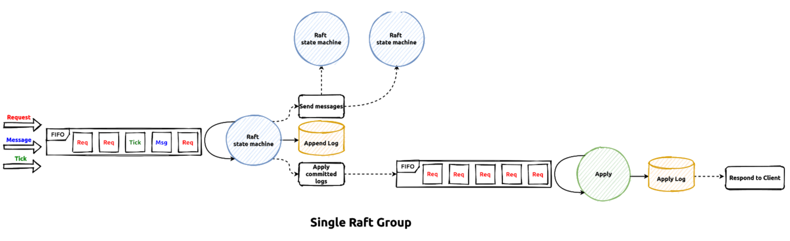
The writes generated by transaction commands will be sent to the raft peer message task queue first, then the raft batch system will poll each raft peer and handle these requests in the raft thread-pool. After all the raft logs are persisted on majority raft group members, they are regarded as commit. Then the correspond apply task be delivered to the apply worker pool to apply the actual write contents to the storage engine, after that the transaction command processing is considered successful and the callback will be invoked to response OK results to the RPC client.
Transaction Record In TiKV
In TiDB, a transaction is considered committed only if its primary key lock is committed successfully (if async commit protocol is not used). The actual key and value written into storage engine is in the following format:
| CF | RocksDB Key | RocksDB Value |
|---|---|---|
| Lock | user_key | lock_info |
| Default | {user_key}{start_ts} | user_value |
| Write | {user_key}{commit_ts} | write_info |
After prewrite, the lock correspond records for the transaction will be written into the storage. Read and write conflicts on the "locked" key will need to consider if it's safe to bypass the lock or it must try to resolve the encountered locks. As commit_ts is part of the stored key, there could be different historical versions for it, and GC is responsible to clean up all the old versions which will not be needed any more. GC mechanism will be introduced in another document.
Transaction Recovery
In TiDB, the transaction coordinator (in tidb-server) is stateless and it will not persist any information. If the transaction coordinator fails for example the tidb-server crashes, the transaction context in memory will get lost, and as the coordinator is gone the normal commit processing will stop. How to recover the transaction state and make a decision if it should commit or abort?
Actually, there is no special mechanism to recover the undetermined-status transactions, the recovery is done by other concurrent conflict transactions, or the conflict transactions will help decide the actual states of the undetermined-status transactions. The lock resolve process will be triggered if the current ongoing transaction encounters locks of other transactions doing reads or writes. The whole resolve process will be introduced in other documents in details.
Transaction Optimizations
Normally the transaction commit will need two phases, the prewrite phase and commit phase. Under certain circumstances transaction commit could be done in a single phase for example the generated transaction mutations could be processed by a single region leader. This optimization is called one-phase commit in TiDB.
The final transaction status is determined by the commit status of the primary key lock, so the response to the client has to wait until the primary key commit has finished. This wait could be saved using the async-commit protocol so the latency of commit processing could be reduced.
They will both be introduced other documents in details.
Summary
This section talks about the brief steps of transaction processing in the TiKV part, and related interfaces, implementations and optimizations.
Optimistic Transaction
Under the optimistic transaction model, modification conflicts are regarded as part of the transaction commit. TiDB cluster uses the optimistic transaction model by default before version 3.0.8, uses pessimistic transaction model after version 3.0.8. System variable tidb_txn_mode controls TiDB uses optimistic transaction mode or pessimistic transaction mode.
This document talks about the implementation of optimistic transaction in TiDB. It is recommended that you have learned about the principles of optimistic transaction.
This document refers to the code of TiDB v5.2.1
Begin Optimistic Transaction
The main function stack to start an optimistic transaction is as followers.
(a *ExecStmt) Exec
(a *ExecStmt) handleNoDelay
(a *ExecStmt) handleNoDelayExecutor
Next
(e *SimpleExec) Next
(e *SimpleExec) executeBegin
The function (e *SimpleExec) executeBegin do the main work for a "BEGIN" statement,The important comment and simplified code is as followers. The completed code is here .
/*
Check the syntax "start transaction read only" and "as of timestamp" used correctly.
If stale read timestamp was set, creates a new stale read transaction and sets "in transaction" state, and return.
create a new transaction and set some properties like snapshot, startTS etc
*/
func (e *SimpleExec) executeBegin(ctx context.Context, s *ast.BeginStmt) error {
if s.ReadOnly {
// the statement "start transaction read only" must be used with tidb_enable_noop_functions is true
// the statement "start transaction read only as of timestamp" can be used Whether tidb_enable_noop_functions is true or false,but that tx_read_ts mustn't be set.
// the statement "start transaction read only as of timestamp" must ensure the timestamp is in the legal safe point range
enableNoopFuncs := e.ctx.GetSessionVars().EnableNoopFuncs
if !enableNoopFuncs && s.AsOf == nil {
return expression.ErrFunctionsNoopImpl.GenWithStackByArgs("READ ONLY")
}
if s.AsOf != nil {
if e.ctx.GetSessionVars().TxnReadTS.PeakTxnReadTS() > 0 {
return errors.New("start transaction read only as of is forbidden after set transaction read only as of")
}
}
}
// process stale read transaction
if e.staleTxnStartTS > 0 {
// check timestamp of stale read correctly
if err := e.ctx.NewStaleTxnWithStartTS(ctx, e.staleTxnStartTS); err != nil {
return err
}
// ignore tidb_snapshot configuration if in stale read transaction
vars := e.ctx.GetSessionVars()
vars.SetSystemVar(variable.TiDBSnapshot, "")
// set "in transaction" state and return
vars.SetInTxn(true)
return nil
}
/* If BEGIN is the first statement in TxnCtx, we can reuse the existing transaction, without the need to call NewTxn, which commits the existing transaction and begins a new one. If the last un-committed/un-rollback transaction is a time-bounded read-only transaction, we should always create a new transaction. */
txnCtx := e.ctx.GetSessionVars().TxnCtx
if txnCtx.History != nil || txnCtx.IsStaleness {
err := e.ctx.NewTxn(ctx)
}
// set "in transaction" state
e.ctx.GetSessionVars().SetInTxn(true)
// create a new transaction and set some properties like snapshot, startTS etc.
txn, err := e.ctx.Txn(true)
// set Linearizability option
if s.CausalConsistencyOnly {
txn.SetOption(kv.GuaranteeLinearizability, false)
}
return nil
}
DML Executed In Optimistic Transaction
There are three kinds of DML operations, such as update, delete and insert. For simplicity, This article only describes the update statement execution process. DML mutations are not sended to tikv directly, but buffered in TiDB temporarily, commit operation make the mutations effective at last.
The main function stack to execute an update statement such as "update t1 set id2 = 2 where pk = 1" is as followers.
(a *ExecStmt) Exec
(a *ExecStmt) handleNoDelay
(a *ExecStmt) handleNoDelayExecutor
(e *UpdateExec) updateRows
Next
(e *PointGetExecutor) Next
(e *UpdateExec) updateRows
The function (e *UpdateExec) updateRows does the main work for update statement. The important comment and simplified code are as followers. The completed code is here .
/*
Take a batch of data that needs to be updated each time.
Traverse every row in the batch, make handle which identifies the data uniquely for the row and generate a new row.
Write the new row to table.
*/
func (e *UpdateExec) updateRows(ctx context.Context) (int, error) {
globalRowIdx := 0
chk := newFirstChunk(e.children[0])
// composeFunc generates a new row
composeFunc = e.composeNewRow
totalNumRows := 0
for {
// call "Next" method recursively until every executor finished, every "Next" returns a batch rows
err := Next(ctx, e.children[0], chk)
// If all rows are updated, return
if chk.NumRows() == 0 {
break
}
for rowIdx := 0; rowIdx < chk.NumRows(); rowIdx++ {
// take one row from the batch above
chunkRow := chk.GetRow(rowIdx)
// convert the data from chunk.Row to types.DatumRow,stored by fields
datumRow := chunkRow.GetDatumRow(fields)
// generate handle which is unique ID for every row
e.prepare(datumRow)
// compose non-generated columns
newRow, err := composeFunc(globalRowIdx, datumRow, colsInfo)
// merge non-generated columns
e.merge(datumRow, newRow, false)
// compose generated columns and merge generated columns
if e.virtualAssignmentsOffset < len(e.OrderedList) {
newRow = e.composeGeneratedColumns(globalRowIdx, newRow, colsInfo)
e.merge(datumRow, newRow, true)
}
// write to table
e.exec(ctx, e.children[0].Schema(), datumRow, newRow)
}
}
}
Commit Optimistic Transaction
Committing transaction includes "prewrite" and "commit" two phases that are explained separately below. The function (c *twoPhaseCommitter) execute does the main work for committing transaction. The important comment and simplified code are as followers. The completed code is here .
/*
do the "prewrite" operation first
if OnePC transaction, return immediately
if AsyncCommit transaction, commit the transaction Asynchronously and return
if not OnePC and AsyncCommit transaction, commit the transaction synchronously.
*/
func (c *twoPhaseCommitter) execute(ctx context.Context) (err error) {
// do the "prewrite" operation
c.prewriteStarted = true
start := time.Now()
err = c.prewriteMutations(bo, c.mutations)
if c.isOnePC() {
// If OnePC transaction, return immediately
return nil
}
if c.isAsyncCommit() {
// commit the transaction Asynchronously and return for AsyncCommit
go func() {
err := c.commitMutations(commitBo, c.mutations)
}
return nil
} else {
// do the "commit" phase
return c.commitTxn(ctx, commitDetail)
}
}
prewrite
The entry function to prewrite a transaction is (c *twoPhaseCommitter) prewriteMutations which calls the function (batchExe *batchExecutor) process to do it. The function (batchExe *batchExecutor) process calls (batchExe *batchExecutor) startWorker to prewrite evenry batch parallelly. The function (batchExe *batchExecutor) startWorker calls (action actionPrewrite) handleSingleBatch to prewrite a single batch.
(batchExe *batchExecutor) process
The important comment and simplified code are as followers. The completed code is here .
// start worker routine to prewrite every batch parallely and collect results
func (batchExe *batchExecutor) process(batches []batchMutations) error {
var err error
err = batchExe.initUtils()
// For prewrite, stop sending other requests after receiving first error.
var cancel context.CancelFunc
if _, ok := batchExe.action.(actionPrewrite); ok {
batchExe.backoffer, cancel = batchExe.backoffer.Fork()
defer cancel()
}
// concurrently do the work for each batch.
ch := make(chan error, len(batches))
exitCh := make(chan struct{})
go batchExe.startWorker(exitCh, ch, batches)
// check results of every batch prewrite synchronously, if one batch fails,
// stops every prewrite worker routine immediately.
for i := 0; i < len(batches); i++ {
if e := <-ch; e != nil {
// Cancel other requests and return the first error.
if cancel != nil {
cancel()
}
if err == nil {
err = e
}
}
}
close(exitCh) // break the loop of function startWorker
return err
}
(batchExe *batchExecutor) startWorker
The important comment and simplified code are as followers. The completed code is here .
// startWork concurrently do the work for each batch considering rate limit
func (batchExe *batchExecutor) startWorker(exitCh chan struct{}, ch chan error, batches []batchMutations) {
for idx, batch1 := range batches {
waitStart := time.Now()
// Limit the number of go routines by the buffer size of channel
if exit := batchExe.rateLimiter.GetToken(exitCh); !exit {
batchExe.tokenWaitDuration += time.Since(waitStart)
batch := batch1
// call the function "handleSingleBatch" to prewrite every batch keys
go func() {
defer batchExe.rateLimiter.PutToken() // release the chan buffer
ch <- batchExe.action.handleSingleBatch(batchExe.committer, singleBatchBackoffer, batch)
}()
} else {
break
}
}
}
(action actionPrewrite) handleSingleBatch
The important comment and simplified code are as followers. The completed code is here .
/*
create a prewrite request and a region request sender that sends the prewrite request to tikv.
(1)get Prewrite Response coming from tikv
(2)If no error happened and it is OnePC transaction, update onePCCommitTS by prewriteResp and return
(3)if no error happened and it is AsyncCommit transaction, update minCommitTS if need and return
(4)If errors hanpped beacause of lock confilict, extract the locks from the error responsed, resolove the locks expired
(5)do the backoff for prewrite
*/
func (action actionPrewrite) handleSingleBatch(c *twoPhaseCommitter, bo *retry.Backoffer, batch batchMutations) (err error) {
// create a prewrite request and a region request sender that sends the prewrite request to tikv.
txnSize := uint64(c.regionTxnSize[batch.region.GetID()])
req := c.buildPrewriteRequest(batch, txnSize)
sender := locate.NewRegionRequestSender(c.store.GetRegionCache(), c.store.GetTiKVClient())
for {
resp, err := sender.SendReq(bo, req, batch.region, client.ReadTimeoutShort)
regionErr, err := resp.GetRegionError()
// get Prewrite Response coming from tikv
prewriteResp := resp.Resp.(*kvrpcpb.PrewriteResponse)
keyErrs := prewriteResp.GetErrors()
if len(keyErrs) == 0 {
// If no error happened and it is OnePC transaction, update onePCCommitTS by prewriteResp and return
if c.isOnePC() {
c.onePCCommitTS = prewriteResp.OnePcCommitTs
return nil
}
// if no error happened and it is AsyncCommit transaction, update minCommitTS if need and return
if c.isAsyncCommit() {
if prewriteResp.MinCommitTs > c.minCommitTS {
c.minCommitTS = prewriteResp.MinCommitTs
}
}
return nil
}// if len(keyErrs) == 0
// If errors hanpped beacause of lock confilict, extract the locks from the error responsed
var locks []*txnlock.Lock
for _, keyErr := range keyErrs {
// Extract lock from key error
lock, err1 := txnlock.ExtractLockFromKeyErr(keyErr)
if err1 != nil {
return errors.Trace(err1)
}
locks = append(locks, lock)
}// for _, keyErr := range keyErrs
// resolve conflict locks expired, do the backoff for prewrite
start := time.Now()
msBeforeExpired, err := c.store.GetLockResolver().ResolveLocksForWrite(bo, c.startTS, c.forUpdateTS, locks)
if msBeforeExpired > 0 {
err = bo.BackoffWithCfgAndMaxSleep(retry.BoTxnLock, int(msBeforeExpired), errors.Errorf("2PC prewrite lockedKeys: %d", len(locks)))
if err != nil {
return errors.Trace(err) // backoff exceeded maxtime, returns error
}
}
}// for loop
}
commit
The entry function of commiting a transaction is (c *twoPhaseCommitter) commitMutations which calls the function (c *twoPhaseCommitter) doActionOnGroupMutations to do it. The batch of primary key will be committed first, then the function (batchExe *batchExecutor) process calls (batchExe *batchExecutor) startWorker to commit the rest batches parallelly and asynchronously. The function (batchExe *batchExecutor) startWorker calls (actionCommit) handleSingleBatch to commit a single batch.
(c *twoPhaseCommitter) doActionOnGroupMutations
The important comment and simplified code are as followers. The completed code is here .
/*
If the groups contain primary, commit the primary batch synchronously
If the first time to commit, spawn a goroutine to commit secondary batches asynchronously
if retry to commit, commit the secondary batches synchronously, because itself is in the asynchronously goroutine
*/
func (c *twoPhaseCommitter) doActionOnGroupMutations(bo *retry.Backoffer, action twoPhaseCommitAction, groups []groupedMutations) error {
batchBuilder := newBatched(c.primary())
// Whether the groups being operated contain primary
firstIsPrimary := batchBuilder.setPrimary()
actionCommit, actionIsCommit := action.(actionCommit)
c.checkOnePCFallBack(action, len(batchBuilder.allBatches()))
// If the groups contain primary, commit the primary batch synchronously
if firstIsPrimary &&
(actionIsCommit && !c.isAsyncCommit()) {
// primary should be committed(not async commit)/cleanup/pessimistically locked first
err = c.doActionOnBatches(bo, action, batchBuilder.primaryBatch())
batchBuilder.forgetPrimary()
}
// If the first time to commit, spawn a goroutine to commit secondary batches asynchronously
// if retry to commit, commit the secondary batches synchronously, because itself is in the asynchronously goroutine
if actionIsCommit && !actionCommit.retry && !c.isAsyncCommit() {
secondaryBo := retry.NewBackofferWithVars(c.store.Ctx(), CommitSecondaryMaxBackoff, c.txn.vars)
c.store.WaitGroup().Add(1)
go func() {
defer c.store.WaitGroup().Done()
e := c.doActionOnBatches(secondaryBo, action, batchBuilder.allBatches())
}
}
else {
err = c.doActionOnBatches(bo, action, batchBuilder.allBatches())
}
return errors.Trace(err)
}
(batchExe *batchExecutor) process
The function (c *twoPhaseCommitter) doActionOnGroupMutations calls (c *twoPhaseCommitter) doActionOnBatches to do the second phase of commit. The function (c *twoPhaseCommitter) doActionOnBatches calls (batchExe *batchExecutor) process to do the main work.
The important comment and simplified code of function (batchExe *batchExecutor) process are as mentioned above in prewrite part . The completed code is here .
(actionCommit) handleSingleBatch
The function (batchExe *batchExecutor) process calls the function (actionCommit) handleSingleBatch to send commit request to all tikv nodes.
The important comment and simplified code are as followers. The completed code is here .
/*
create a commit request and commit sender.
If regionErr happened, backoff and retry the commit operation.
If the error is not a regionErr, but rejected by TiKV beacause the commit ts was expired, retry with a newer commits.
Other errors happened, return error immediately.
No error happened, exit the for loop and return success.
*/
func (actionCommit) handleSingleBatch(c *twoPhaseCommitter, bo *retry.Backoffer, batch batchMutations) error {
// create a commit request and commit sender
keys := batch.mutations.GetKeys()
req := tikvrpc.NewRequest(tikvrpc.CmdCommit, &kvrpcpb.CommitRequest{
StartVersion: c.startTS,
Keys: keys,
CommitVersion: c.commitTS,
}, kvrpcpb.Context{Priority: c.priority, SyncLog: c.syncLog,
ResourceGroupTag: c.resourceGroupTag, DiskFullOpt: c.diskFullOpt})
tBegin := time.Now()
attempts := 0
sender := locate.NewRegionRequestSender(c.store.GetRegionCache(), c.store.GetTiKVClient())
for {
attempts++
resp, err := sender.SendReq(bo, req, batch.region, client.ReadTimeoutShort)
regionErr, err := resp.GetRegionError()
// If regionErr happened, backoff and retry the commit operation
if regionErr != nil {
// For other region error and the fake region error, backoff because there's something wrong.
// For the real EpochNotMatch error, don't backoff.
if regionErr.GetEpochNotMatch() == nil || locate.IsFakeRegionError(regionErr) {
err = bo.Backoff(retry.BoRegionMiss, errors.New(regionErr.String()))
if err != nil {
return errors.Trace(err)
}
}
same, err := batch.relocate(bo, c.store.GetRegionCache())
if err != nil {
return errors.Trace(err)
}
if same {
continue
}
err = c.doActionOnMutations(bo, actionCommit{true}, batch.mutations)
return errors.Trace(err)
}// if regionErr != nil
// If the error is not a regionErr, but rejected by TiKV beacause the commit ts was expired, retry with a newer commits. Other errors happened, return error immediately.
commitResp := resp.Resp.(*kvrpcpb.CommitResponse)
if keyErr := commitResp.GetError(); keyErr != nil {
if rejected := keyErr.GetCommitTsExpired(); rejected != nil {
// 2PC commitTS rejected by TiKV, retry with a newer commits, update commit ts and retry.
commitTS, err := c.store.GetTimestampWithRetry(bo, c.txn.GetScope())
c.mu.Lock()
c.commitTS = commitTS
c.mu.Unlock()
// Update the commitTS of the request and retry.
req.Commit().CommitVersion = commitTS
continue
}
if c.mu.committed {
// 2PC failed commit key after primary key committed
// No secondary key could be rolled back after it's primary key is committed.
return errors.Trace(err)
}
return err
}
// No error happened, exit the for loop
break
}// for loop
}
Lock Resolver
As we described in other sections, TiDB's transaction system is based on Google's Percolator algorithm. Which makes it necessary to resolve locks when a reading transaction meets locked keys or during GC.
So we introduced Lock Resolver in TiDB to resolve locks.
The Data Structure
Lock Resolver is a quiet simple struct:
type LockResolver struct {
	store storage
	mu    struct {
		sync.RWMutex
		// resolved caches resolved txns (FIFO, txn id -> txnStatus).
		resolved       map[uint64]TxnStatus
		recentResolved *list.List
	}
}
The store field is used to send requests to a region on TiKV.
And the fields inside the mu are used to cache the resolved transactions' status, which is used to speed up the transaction status checking.
Lock Resolving process
Now let's see the real important part: the lock resolving process.
Basically, the resolving process is in 2 steps:
- For each lock, get the commit status of the corresponding transaction.
- Send
ResolveLockcmd to tell the storage layer to do the resolve work.
In the following several paragraphs, we will give you some brief introduction about each step.
If you want to read all of the code, LockResolver.resolveLocks is a good place to start.
Get transaction status for a lock
TiDB part
Related code is LockResolver.getTxnStatusFromLock and LockResolver.getTxnStatus.
LockResolver.getTxnStatus just assemble a CheckTxnStatus request and send it to the TiKV the primary key is located on. TiKV will return a TxnStatus, which represents the status of a transaction, like RolledBack(the transaction has already been rolled back before), TtlExpire(the transaction's is expired, TiKV just rolled it back), Committed(the transaction was committed successfully before), etc. to TiDB.
LockResolver.getTxnStatusFromLock basically delegate its work to LockResolver.getTxnStatus with the information in the lock and add some retry and error handling logic.
TiKV part
As we showed above, we use a CheckTxnStatus request to get the status of a transaction when resolving a lock.
The major processing logic can be found here, this function is a little complex (mainly because the scheduling process in TiKV), I'll show you the basic idea with some simplified pseudo code with detailed comments, before that, there are several optimizations and related concepts we should know:
collapse continuous rollbacks (tikv#3290)
Instead of keeping all rollbacks in write column family when a key rollbacked for several times, this PR collapse continuous rollbacks, and only keep the latest rollback.
protect primary locks (tikv#5575)
After we have pessimistic lock in TiKV, if the rollback record of the primary lock is collapsed and TiKV receives stale acquire_pessimistic_lock and prewrite, the transaction will commit successfully even if secondary locks are rolled back. To solve this problem, we can prevent the rollback records of the primary key of pessimistic transactions from being collapsed. By setting the short value of these rollback records to "protected".
gc_fence (tikv#9207)
See the super detailed comment here.
After understand these, you can finally understand the code:
fn process_write(self, snapshot: Snapshot, context: WriteContext) {
	// async commit related stuff, see async commit doc
	context.concurrency_manager.update_max_ts();

	let lock = load_lock_on(self.primary_key);

	let (txn_status, released) = if let Some(lock) = lock && lock.ts == self.lock_ts {
		// the lock still exists, ie. the transaction is still alive
		check_txn_status_lock_exists();
	} else {
		// the lock is missing
		check_txn_status_missing_lock();
	}

	if let TxnStatus::TtlExpire = txn_status {
        context.lock_mgr.notify_released(released);
    }

	// return result to user
	return txn_status;
}
fn check_txn_status_lock_exists(
	primary_key: Key,
	lock: Lock,
) {
	if use_async_commit {
		return (TxnStatus::Uncommitted, None)
	}
	let lock_expired = lock.ts.physical() + lock.ttl < current_ts.physical()
	if lock_expired {
		if resolving_pessimistic_lock && lock.lock_type == LockType::Pessimistic {
			// unlock_key just delete `primary_key` in lockCF
            let released = unlock_key(primary_key);
            return (TxnStatus::PessimisticRollBack, released);
        } else {
			// rollback_lock is complex, see below
            let released = rollback_lock(lock);
            return (TxnStatus::TtlExpire, released);
        }
	}
	return (TxnStatus::Uncommitted, None)
}
pub fn rollback_lock() {
	// get transaction commit record on `key`
	let commit_record = get_txn_commit_record(key);
    let overlapped_write = match commit_record {
		// The commit record of the given transaction is not found.
		// But it's possible that there's another transaction's commit record, whose `commit_ts` equals to the current transaction's `start_ts`. That kind of record will be returned via the `overlapped_write` field.
    	// In this case, if the current transaction is to be rolled back, the `overlapped_write` must not be overwritten.
        TxnCommitRecord::None { overlapped_write } => overlapped_write,
        TxnCommitRecord::SingleRecord { write, .. } if write.write_type != WriteType::Rollback => {
            panic!("txn record found but not expected: {:?}", txn)
        }
        _ => return txn.unlock_key(key, is_pessimistic_txn),
    };

    // If prewrite type is DEL or LOCK or PESSIMISTIC, it is no need to delete value.
    if lock.short_value.is_none() && lock.lock_type == LockType::Put {
        delete_value(key, lock.ts);
    }

	// if this is primary key of a pessimistic transaction, we need to protect the rollback just as we mentioned above
	let protect = is_pessimistic_txn && key.is_encoded_from(&lock.primary);
	put_rollback_record(key, protect);
	collapse_prev_rollback(key);
    return unlock_key(key, is_pessimistic_txn);
}
pub fn check_txn_status_missing_lock() {
    match get_txn_commit_record(primary_key) {
        TxnCommitRecord::SingleRecord { commit_ts, write } => {
            if write.write_type == WriteType::Rollback {
                Ok(TxnStatus::RolledBack)
            } else {
                Ok(TxnStatus::committed(commit_ts))
            }
        }
        TxnCommitRecord::OverlappedRollback { .. } => Ok(TxnStatus::RolledBack),
        TxnCommitRecord::None { overlapped_write } => {
            if MissingLockAction::ReturnError == action {
                return Err(TxnNotFound);
            }
            if resolving_pessimistic_lock {
                return Ok(TxnStatus::LockNotExistDoNothing);
            }

            let ts = reader.start_ts;

            if action == MissingLockAction::Rollback {
                collapse_prev_rollback(txn, reader, &primary_key)?;
            }

            if let (Some(l), None) = (mismatch_lock, overlapped_write.as_ref()) {
				// When putting rollback record on a key that's locked by another transaction, the second transaction may overwrite the current rollback record when it's committed. Sometimes it may break consistency.
				// To solve the problem, add the timestamp of the current rollback to the lock. So when the lock is committed, it can check if it will overwrite a rollback record by checking the information in the lock.
                mark_rollback_on_mismatching_lock(
                    &primary_key,
                    l,
                    action == MissingLockAction::ProtectedRollback,
                );
            }

            // Insert a Rollback to Write CF in case that a stale prewrite
            // command is received after a cleanup command.
			put_rollback_record(primary_key, action == MissingLockAction::ProtectedRollback);

            Ok(TxnStatus::LockNotExist)
        }
    }
}
Resolve
TiDB Part
After we get the transaction status with LockResolver.getTxnStatusFromLock here, if the transaction has been expired (either committed or rollbacked), we need to resolve the lock.
There are three different kinds of locks we need to pay attention to when doing the resolving work:
- locks created by async commit transactions
This kind of lock will be resolved by
resolveLockAsyncfunction, you can refer to Transaction recovery chapter in async commit for more information. - pessimistic locks created by pessimistic transaction
This kind of lock will be resolved by
resolvePessimisticLockfunction, which just sendPessimisticRollbackRequestto TiKV, with some retry and error handling logic. - optimistic locks created by optimistic transaction
This kind of lock will be resolved by
resolveLockfunction, which just sendResolveLockRequestto TiKV, with some retry and error handling logic.
TiKV Part
When a resolve lock request reaches TiKV, depends on whether resolve_keys field is empty or not, TiKV will do different things:
ResolveLockReadPhase + ResolveLock
This will triggered when resolve_keys field is not set.
ResolveLockReadPhase will scan keys and locks on them which should be resolved in a region, to prevent huge writes, we'll do the scan in batches (RESOLVE_LOCK_BATCH_SIZE keys in a batch).
After each batch is read, a ResolveLock command will be spawned to do the real resolve work.
In ResolveLock, for each key and lock on it, depend on whether the transaction status
is committed or not, we'll cleanup or commit it.
And then, TiKV will wake up the blocked transactions, and we are done.
ResolveLockLite
This will triggered when resolve_keys field is set.
ResolveLockLite is just a simplified version of ResolveLock, which will do the resolve work on resolve_keys on the request.
Where do we use it?
- When acquiring PessimisticLock, it is possible that a transaction meet other transaction's lock when it is trying to acquire the lock. In this situation, we should try to resolve the old transaction's lock first.
- When reading from TiKV, eg. when scanning data, we should resolve the lock we met first.
- When doing GC, see the GC chapter for detail.
Summary
This document talked about the data structure of Lock Resolver in TiDB, and its working process and usage. You can combine this with other parts of our transaction system to have a deeper understanding.
Pessimistic Transaction
Async Commit
Async commit is an optimization of two phase commit introduced in TiDB 5.0. The optimization greatly reduces the latency of the two phase commit process.
This document talks about the implementation of async commit in TiDB. It is recommended that you have learned about the theories of async commit first.
This document refers to the code of TiDB v5.2.1, the corresponding client-go and TiKV v5.2.1.
TiDB part
Preparations
Async commit does not change the behavior during transaction execution. The changes begin from 2PC execution.
Because we need to record the key list in the primary lock, it is not suitable to use the async commit protocol for large transactions. And binlog does not support async commit, so we disable async commit if binlog is enabled. These checks can be found here.
And in the theory blog, we proves that using a latest timestamp from PD can guarantee linearizability. You can find the code here. Actually, it is not always necessary to get this timestamp, the comment here explains it:
// priority of the sysvar is lower than `start transaction with causal consistency only`
if val := s.txn.GetOption(kv.GuaranteeLinearizability); val == nil || val.(bool) {
    // We needn't ask the TiKV client to guarantee linearizability for auto-commit transactions
    // because the property is naturally holds:
    // We guarantee the commitTS of any transaction must not exceed the next timestamp from the TSO.
    // An auto-commit transaction fetches its startTS from the TSO so its commitTS > its startTS > the commitTS
    // of any previously committed transactions.
    s.txn.SetOption(kv.GuaranteeLinearizability,
                    sessVars.TxnCtx.IsExplicit && sessVars.GuaranteeLinearizability)
}
Later, we also calculate a maxCommitTS. This will be discussed later in the DDL compatibility part.
Prewrite
If we decide to use async commit, we need to provide some extra information to enable the async commit protocol, the UseAsyncCommit flag and the secondary keys:
req := &kvrpcpb.PrewriteRequest{/* ommitted */}
if c.isAsyncCommit() {
    if batch.isPrimary {
        req.Secondaries = c.asyncSecondaries()
    }
    req.UseAsyncCommit = true
}
If the prewriting succeeds, there are two cases.
If TiKV cannot proceed the async-commit protocol successfully, (probably because the calculated commit TS exceeds maxCommitTS), we fallback to the traditional percolator protocol. Otherwise, the prewrite request succeeds, so we can update the global MinCommitTS.
// 0 if the min_commit_ts is not ready or any other reason that async
// commit cannot proceed. The client can then fallback to normal way to
// continue committing the transaction if prewrite are all finished.
if prewriteResp.MinCommitTs == 0 {
    c.setAsyncCommit(false)
} else {
    c.mu.Lock()
    if prewriteResp.MinCommitTs > c.minCommitTS {
        c.minCommitTS = prewriteResp.MinCommitTs
    }
    c.mu.Unlock()
}
However, if any response of prewrite is finally lost due to RPC reasons, it is impossible for us to know whether the prewriting succeeds. And it also means we cannot know whether the transaction succeeds. In this case, we can only return an "undetermined error" and the client connection will be closed:
defer func() {
    if err != nil {
        // If we fail to receive response for async commit prewrite, it will be undetermined whether this
        // transaction has been successfully committed.
        // If prewrite has been cancelled, all ongoing prewrite RPCs will become errors, we needn't set undetermined
        // errors.
        if (c.isAsyncCommit() || c.isOnePC()) && sender.GetRPCError() != nil && atomic.LoadUint32(&c.prewriteCancelled) == 0 {
            c.setUndeterminedErr(errors.Trace(sender.GetRPCError()))
        }
    }
}()
But don't worry, this does not happen very often. It is safe to retry a prewrite which temporarily fails due to network reasons. The above problem only happens if a prewrite request has been sent, but later retries all fail due to RPC errors.
Commit
The whole commit process is done asynchronously in background. This is why the optimization is called "async commit":
if c.isAsyncCommit() {
    // For async commit protocol, the commit is considered success here.
    c.txn.commitTS = c.commitTS
    go func() {
        commitBo := retry.NewBackofferWithVars(c.store.Ctx(), CommitSecondaryMaxBackoff, c.txn.vars)
        c.commitMutations(commitBo, c.mutations)
    }()
    return nil
}
It does not matter even if some temporary error happens in the commit process. Anyone who encounters these uncommitted async-commit locks is able to finally commit them. Next, we will talk about this.
Transaction recovery
If a reader encounters an expired async-commit lock, it needs to resolve this lock.
As usual, the primary lock is checked first to get the transaction information. If it is using the async-commit protocol, the primary lock is never cleaned in CheckTxnStatus. Then we call the resolveLockAsync function to resolve this transaction.
First, it checks all secondary locks. After that we should know the commit TS of this transaction. If all locks exist or some key has been committed, we can calculate a real commit TS. And if some lock does not exist, the commit TS is zero which indicates the transaction should be rolled back.
resolveData, err := lr.checkAllSecondaries(bo, l, &status)
if err != nil {
    return err
}
status.commitTS = resolveData.commitTs
Then we can use this commit TS to resolve all the locks in this transaction.
Another case is when the transaction is actually not an async-commit transaction. Some keys are prewritten with the async-commit protocol while some keys fail and fallback. Such a case can be detected when checking secondary locks:
if !lockInfo.UseAsyncCommit {
    return &nonAsyncCommitLock{}
}
And then, we will retry the lock resolving process assuming the transaction is not an async-commit transaction. And now, CheckTxnStatus can clean up an expired primary lock:
if _, ok := errors.Cause(err).(*nonAsyncCommitLock); ok {
    err = resolve(l, true)
}
DDL compatibility
Without async commit, we check whether the schema changes before the second phase of the commit. But as the transaction is committed after prewriting all the locks, we don't have the chance to check the schema version. Here we use a trick to work around the problem.
For DDLs which involve data reorganizations, we delay 3 seconds by default. Then, before doing 2PC, we set MaxCommitTS to 2 seconds later from now:
func (c *twoPhaseCommitter) calculateMaxCommitTS(ctx context.Context) error {
	// Amend txn with current time first, then we can make sure we have another SafeWindow time to commit
	currentTS := oracle.ComposeTS(int64(time.Since(c.txn.startTime)/time.Millisecond), 0) + c.startTS
	_, _, err := c.checkSchemaValid(ctx, currentTS, c.txn.schemaVer, true)
	if err != nil {
		return errors.Trace(err)
	}

	safeWindow := config.GetGlobalConfig().TiKVClient.AsyncCommit.SafeWindow
	maxCommitTS := oracle.ComposeTS(int64(safeWindow/time.Millisecond), 0) + currentTS

	c.maxCommitTS = maxCommitTS
	return nil
}
Therefore, all async-commit transaction using the old schema should be committed before DDL reorganization happens. So, the DDL reorganization will not miss these data.
TiKV part
Concurrency manager
As discussed in the theory blog, TiKV needs to record the max TS and set some memory locks for ongoing prewrite requests.
For simplicity, we use a global component to implement it. We call it the "concurrency manager".
The methods provided by the concurrency manager can be found in this file.
It is very easy to update the max TS. It's just an atomic operation:
#![allow(unused)]
fn main() {
pub fn update_max_ts(&self, new_ts: TimeStamp) {
    if new_ts != TimeStamp::max() {
        self.max_ts.fetch_max(new_ts.into_inner(), Ordering::SeqCst);
    }
}
}
It is a bit complex for memory locks.
The memory locks can have multiple accessors. Of course, the first one is the prewrite process. And because all readers need to check the memory locks, they are accessors of the memory locks, too. The locks can be removed from the table when there are no accessors.
So the memory table just owns a weak reference to the lock. We define the table like this:
#![allow(unused)]
fn main() {
pub struct LockTable(pub Arc<SkipMap<Key, Weak<KeyHandle>>>);
}
To add a memory lock and be able to write lock information, the lock_key method needs to be called to get a lock guard. The locking process is a bit tricky to handle various possiblities in the multi-thread environment. If interested, you can refer to the code for details.
Prewrite
The code of prewrite can be found here. We will talk about some key points in the code about async commit.
In TiKV, secondary_keys and try_one_pc in the prewrite request are used to determine the type of the prewrite:
#![allow(unused)]
fn main() {
let commit_kind = match (&self.secondary_keys, self.try_one_pc) {
    (_, true) => CommitKind::OnePc(self.max_commit_ts),
    (&Some(_), false) => CommitKind::Async(self.max_commit_ts),
    (&None, false) => CommitKind::TwoPc,
};
}
Only when prewriting the primary lock, secondary locks need to be written in the lock:
#![allow(unused)]
fn main() {
let mut secondaries = &self.secondary_keys.as_ref().map(|_| vec![]);
if Some(m.key()) == async_commit_pk {
    secondaries = &self.secondary_keys;
}
}
In the prewrite action, async commit does not change the checks. What is different is in the write_lock function.
Besides setting secondary keys in the primary lock, it calls async_commit_timestamps to set min_commit_ts in the lock.
Here is the simplified code:
#![allow(unused)]
fn main() {
let final_min_commit_ts = key_guard.with_lock(|l| {
    let max_ts = txn.concurrency_manager.max_ts();

    let min_commit_ts = cmp::max(cmp::max(max_ts, start_ts), for_update_ts).next();
    let min_commit_ts = cmp::max(lock.min_commit_ts, min_commit_ts);

    let max_commit_ts = max_commit_ts;
    if (!max_commit_ts.is_zero() && min_commit_ts > max_commit_ts) {
        return Err(ErrorInner::CommitTsTooLarge {
            start_ts,
            min_commit_ts,
            max_commit_ts,
        });
    }

    lock.min_commit_ts = min_commit_ts;
    *l = Some(lock.clone());
    Ok(min_commit_ts)
})?;

txn.guards.push(key_guard);
}
The final min_commit_ts is set to the maximum of (max TS + 1) and the original min_commit_ts. And if the min_commit_ts is greater than max_commit_ts, a CommitTsTooLarge is returned and triggers a fallback to non-async commit.
The operation is done while locked to guarantee the atomicity of getting the max TS and setting the min_commit_ts in the lock.
The key guard is saved until the lock is successfully written into RocksDB. Before that, readers are able to check the locks in order not to break any constraint. We can release the guard to remove the lock in the memory table after the readers can read the lock from the RocksDB.
Fallback to non-async commit
The client may provide a max_commit_ts constraint. If the calculated min_commit_ts is larger than the max_commit_ts, we need to fallback to non-async commit.
When the CommitTsTooLarge error happens, the lock will still be written, but in the lock there will be no use_async_commit flag and no secondary keys will be recorded:
#![allow(unused)]
fn main() {
if let Err(Error(box ErrorInner::CommitTsTooLarge { .. })) = &res {
    lock.use_async_commit = false;
    lock.secondaries = Vec::new();
}
}
After any key encounters this error, we don't need to do async commit prewrite for later keys:
#![allow(unused)]
fn main() {
 Err(MvccError(box MvccErrorInner::CommitTsTooLarge { .. })) | Ok((..)) => {
    // fallback to not using async commit or 1pc
    props.commit_kind = CommitKind::TwoPc;
    async_commit_pk = None;
    self.secondary_keys = None;
    // release memory locks
    txn.guards = Vec::new();
    final_min_commit_ts = TimeStamp::zero();
}
}
When any key in a transaction fallbacks to non-async commit mode, the transaction will be considered as a non-async commit transaction.
Memory lock checking
All transactional reading requests need to update max TS and check memory locks. If the min_commit_ts of the lock is not larger than the snapshot timestamp of the reading, it is not safe to proceed this read. Then, an error will be returned and the client needs to retry later.
Here is an example in the storage module:
#![allow(unused)]
fn main() {
// Update max_ts and check the in-memory lock table before getting the snapshot
if !pb_ctx.get_stale_read() {
    concurrency_manager.update_max_ts(start_ts);
}
let isolation_level = pb_ctx.get_isolation_level();
if isolation_level == IsolationLevel::Si {
    for key in keys.clone() {
        concurrency_manager
            .read_key_check(key, |lock| {
                Lock::check_ts_conflict(Cow::Borrowed(lock), key, start_ts, bypass_locks)
            })
            .map_err(|e| txn::Error::from_mvcc(e))?;
    }
}
}
Check transaction status
We use CheckTxnStatus to get the status of the primary lock and use CheckSecondaryLocks for secondary locks.
In CheckTxnStatus, we cannot remove the primary lock simply because it is expired because the transaction may have prewritten all the locks. So we always just return the lock information for async commit locks:
#![allow(unused)]
fn main() {
if lock.use_async_commit {
    if force_sync_commit {
        // The fallback case
    } else {
        return Ok((TxnStatus::uncommitted(lock, false), None));
    }
}
}
The idea of CheckSecondaryLocks is simple. If any lock in the list of secondary keys does not exist, remove the lock and write rollback if necessary. And if any lock has been committed, the transaction is committed. You can refer to its implementation for details.
Update max TS on region changes
In TiKV, we must guarantee that when a key is prewritten using the async-commit protocol, all readings at this key have updated the max TS. Now we update the max TS on the local TiKV. But there are some other cases we missed. If the reading happens on other TiKVs, then the region leader is transfered to the current TiKV or the region is merged into a region whose leader is on this TiKV, the max TS can be incorrect.
So, for safety, we choose to get a latest timestamp from PD when a region becomes leader or a region is merged.
Before the max TS is updated, the corresponding region is not allowed to proceed an async-commit prewrite. The property is checked here.
Summary
This is how the "async commit" optimization is implemented in TiDB.
Due to limited space, some subtle problems such as non-unique timestamps and the compatibility with follower read are not involved.
During the implementation of async commit, many problems blocking one-phase commit (1PC) are solved. So it becomes relatively easy to implement 1PC in TiDB. The next document will introduce the implementation details of 1PC.
1PC
Along with async commit, there is another optimization for transactions, namely 1PC. That is, for transactions that all keys can be prewritten in a single prewrite request to TiKV, we can commit it immediately while prewriting, skipping the second phase (the commit phase) completely. This reduces latency and improves throughput in scenarios where there are many small and simple transactions.
Before working on development related to 1PC, it's recommended to understand how 1PC (as well as async commit) works, and how async commit is implemented (since 1PC is implemented based on async commit). It's recommended to read these two articles first, and this article assumes you already know about them:
- This article is a great material to learn about the overall idea of async commit and 1PC.
- This article explains the code related to async commit.
RPC Protocol
A few additional fields to the Prewrite RPC messages are needed for 1PC.
message PrewriteRequest {
    // ...
    bool try_one_pc = 13;
    uint64 max_commit_ts = 14;
}

message PrewriteResponse {
    // ...
    uint64 one_pc_commit_ts = 4;
}
- The
try_one_pcfield in the request is to tell TiKV that when handling the prewrite request, it needs to try to commit it directly in 1PC if possible. - The
max_commit_tsis used by 1PC and async commit in common. It limits the maximum allowed commit ts. It's related to a mechanism to avoid a transaction commits while schema changed between the transaction's start_ts and commit_ts. This is mechanism is already explained in the article about async commit. - When TiKV successfully commits a transaction in 1PC, the
one_pc_commit_tsfield in thePrewriteResponsewill be set to tell TiDB the final commit_ts. Sometimes TiKV may fail to commit the transaction by 1PC, but it's able to prewrite it in normal 2PC way. In this case, theone_pc_commit_tswill be zero to indicate that TiDB still needs to proceed on the 2PC procedure (i.e. the commit phase of 2PC).
TiDB Part
Based on the implementation of normal 2PC and async commit, there isn't too much additional code to support 1PC, but the code changes are scattered.
The core of 2PC logic is in twoPhaseCommitter, and the entry is the execute method. You might already know about it from previous articles. But since the path from the execute function to sending RPC requests is quite complicated, let's see how the overall control flow looks like:
execute- ⭐
checkOnePC prewriteMutationsdoActionOnMutations- ⭐
checkOnePCFallBack doActionOnGroupMutations- Divide mutations into batches
- ⭐
checkOnePCFallBack doActionOnBatchesactionPrewrite.handleSingleBatchbuildPrewriteRequestSendReq- ⭐ Error handling (maybe fallback, maybe retry
doActionOnMutationsrecursively)
- ⭐
- If not committed in 1PC, continue 2PC or async commit procedure.
- ⭐
The starred items are the ones we are interested in in this article.
Checking if 1PC Can Be Used
In the execute method, it checks if 1PC can be used just after checking async commit, before performing any crucial part of the transaction procedure:
func (c *twoPhaseCommitter) checkOnePC() bool {
    // Disable 1PC in local transactions. This is about another feature that's not compatible with
    // async and 1PC, where transactions have two different "scopes" namely Global and Local.
    if c.txn.GetScope() != oracle.GlobalTxnScope {
        return false
    }

    return !c.shouldWriteBinlog() && c.txn.enable1PC // `txn` is the `KVTxn` object and the value of
                                                     // `enable1PC` is passed from Session previously.
}

func (c *twoPhaseCommitter) execute(ctx context.Context) (err error) {
    // ...

    // Check if 1PC is enabled.
    if c.checkOnePC() {
        commitTSMayBeCalculated = true
        c.setOnePC(true)
        c.hasTriedOnePC = true
    }

    // ...
}
Same as async commit, 1PC can't be enabled when using TiDB-Binlog.
Note that we still don't know how many prewrite requests this transaction needs. It will be checked later.
Also note that the checkOnePC function doesn't check the transaction's size like how async commit does. Actually, the transaction size is implicitly limited when the keys are divided into batches during prewrite phase.
The logic then goes to the prewriteMutation function from here, which then calls the doActionOnMutations function:
func (c *twoPhaseCommitter) doActionOnMutations(bo *retry.Backoffer, action twoPhaseCommitAction, mutations CommitterMutations) error {
	if mutations.Len() == 0 {
		return nil
	}
	groups, err := c.groupMutations(bo, mutations)
	if err != nil {
		return errors.Trace(err)
	}

	// This is redundant since `doActionOnGroupMutations` will still split groups into batches and
	// check the number of batches. However we don't want the check fail after any code changes.
	c.checkOnePCFallBack(action, len(groups))

	return c.doActionOnGroupMutations(bo, action, groups)
}
This function divides the mutations by regions, which means, mutations to keys that belong to the same region are grouped together. Then it calls the doActionOnGroupMutations function:
func (c *twoPhaseCommitter) doActionOnGroupMutations(bo *retry.Backoffer, action twoPhaseCommitAction, groups []groupedMutations) error {
	// ...

	batchBuilder := newBatched(c.primary())
	for _, group := range groups {
		batchBuilder.appendBatchMutationsBySize(group.region, group.mutations, sizeFunc, txnCommitBatchSize)
	}
	firstIsPrimary := batchBuilder.setPrimary()

	// ...

	c.checkOnePCFallBack(action, len(batchBuilder.allBatches()))

    // ...
doActionOnGroupMutations divides each group into multiple batches if the group has too many keys.
Note that these two functions both call a function named checkOnePCFallBack. It's a helper to check if the transaction needs more than one request to finish prewrite. If so, the 1PC flag will be set to false and 1PC will be disabled for this transaction.
Sending RPC Requests
After the procedure stated above, the control flow goes to the handleSingleBatch method of the actionPrewrite type. Then there's nothing complicated. It creates an RPC request for prewrite, and the try_one_pc field of the request will be set according to whether 1PC is still enabled after the previous procedure. For a 1PC transaction, once sender.Send is invoked and nothing goes wrong, it means the transaction is successfully committed by 1PC. Finally, the execute function will return without running the 2PC commit.
Error Handling and Falling Back
However, there are chances that something goes wrong. There are multiple possible cases, some of which needs to be paid attention of:
Region Error
A region error means the region may have been changed, including merging and splitting, therefore the request is invalid since it's using an outdated region information.
Suppose we are trying to do prewrite for a 1PC transaction and encountered a region error. The keys in the transaction were located in a single region before, thus 1PC can be used. But the region's state has already changed, so the keys may be located in more than one new regions, if region splitting has happened.
However, we don't need any extra code to handle it for 1PC in this case. That's because on region error, it will retry recursively, where checkOnePCFallBack will be invoked again. So in the stated above, the checkOnePCFallBack call will unset the 1PC flag while retrying.
Fallen Back by TiKV
When TiKV receives a prewrite request with try_one_pc flag set, sometimes it's possible that TiKV cannot commit it directly in 1PC. In this case TiKV will perform a normal prewrite, and return a response with one_pc_commit_ts = 0 to indicate that the transaction is not committed in 1PC way. Then, TiDB will continue normal 2PC procedure.
Currently, the only possible case that this fallback happens is that the calculated min_commit_ts exceeds our max_commit_ts, therefore neither 1PC nor async commit can be used. The handling logic is here.
RPC Error
If we cannot receive an RPC response after a few retries, same as that in async commit, there will be an undetermined error that will close the client connection.
Recovery
When a 2PC transaction crashes on the half way, we need some mechanism to know the transaction's final state (committed or rolled back). For a 1PC transaction, things are much simpler: since TiKV performs the 1PC writing atomically, so the transaction must be either not-prewritten state or fully committed state. In other words, a 1PC transaction won't leave any lock after a crash. Therefore, nothing about 1PC transactions needs recovery.
TiKV Part
1PC and async commit face the same challenges: commit_ts calculation, follower read consistency, etc. Therefore, 1PC and async commit share many code, including the concurrency manager and many logic in the prewrite procedure.
1PC transaction fetches the max_ts for min_commit_ts calculation and acquires the memory lock in the concurrency manager in the same way as how async commit does. The falling back logic is also using the same code as async commit. For details about them, please refer to the article of async commit.
The only notable difference from async commit is what data is being written after the prewrite request.
First, here the txn object buffers data in a different way from non-1PC transaction:
#![allow(unused)]
fn main() {
// impl MvccTxn
pub(crate) fn put_locks_for_1pc(&mut self, key: Key, lock: Lock, remove_pessimstic_lock: bool) {
    self.locks_for_1pc.push((key, lock, remove_pessimstic_lock));
}
}
Different from the normal put_locks function, locks are not serialized into bytes at this time. Neither are them immediately converted to Write records. It's because we don't know how they should be serialized until all keys are processed. While we expect the keys will be committed by 1PC, it's also possible that we find they need to fallback to 2PC later, in which case the locks will be converted to normal 2PC locks.
Then, If we don't see any error after processing all keys, the locks recorded by the put_locks_for_1pc function will be converted into Write records, and the final min_commit_ts will be used as the commit_ts (here and here):
#![allow(unused)]
fn main() {
/// Commit and delete all 1pc locks in txn.
fn handle_1pc_locks(txn: &mut MvccTxn, commit_ts: TimeStamp) -> ReleasedLocks {
    let mut released_locks = ReleasedLocks::new(txn.start_ts, commit_ts);

    for (key, lock, delete_pessimistic_lock) in std::mem::take(&mut txn.locks_for_1pc) {
        let write = Write::new(
            WriteType::from_lock_type(lock.lock_type).unwrap(),
            txn.start_ts,
            lock.short_value,
        );
        // Transactions committed with 1PC should be impossible to overwrite rollback records.
        txn.put_write(key.clone(), commit_ts, write.as_ref().to_bytes());
        if delete_pessimistic_lock {
            released_locks.push(txn.unlock_key(key, true));
        }
    }

    released_locks
}
}
Note the special handling about delete_pessimistic_lock. If the transaction is a pessimistic transaction, there may already be pessimistic locks when we are performing Prewrite. Since we will write the Write record instead of overwriting the lock, if there's a pessimistic lock, it need to be deleted.
Summary
Based on the work already done by async commit, there's not much code introduced by 1PC. 1PC faced a lot of tricky challenges that async commit meets too, and therefore the implementation of 1PC and async commit shares many common code. If you understand how async commit works, 1PC will not be too hard to understand.
MVCC Garbage Collection
TiDB is a database built on TiKV, a multi-version storage engine which supports Snapshot Isolation(SI) based on the MultiVersion Concurrency Control (MVCC). Semantically, a multi-version system keeps multi copies of data. However, in the long-term running, there will be many garbage data that takes up a lot of disk space as well as has an impact on performance. A GC is responsible for cleaning up unused data and free the space while minimizing the impact on the system. This document talks about how MVCC GC works and implements in TiDB.
This document refers to the code of TiDB v5.2.1, PD v5.2.1, and TiKV v5.2.1.
TiDB part
You probably already know that data is stored in TiKV instances in a TiDB cluster. However, the GC process should be triggered by TiDB because it's the coordinator of the cluster. There are several requirements for TiDB when triggering GC.
- Clean up as much garbage data as possible.
- Any data that is possibly read by opened transactions should be kept.
- GC should not be frequently triggered.
There is an inner table named mysql.tidb in TiDB which stores many runtime information. Actually, these variables are stored in TiKV as common KV variables. We'll talk about the usage of these variables in the GC workflow later.
MySQL [test]> select * from mysql.tidb where variable_name like "tikv_gc_%";
+--------------------------+----------------------------------------------------------------------------------------+---------------------------------------------------------------------------------------------+
| VARIABLE_NAME            | VARIABLE_VALUE                                                                         | COMMENT                                                                                     |
+--------------------------+----------------------------------------------------------------------------------------+---------------------------------------------------------------------------------------------+
| tikv_gc_leader_uuid      | 5f0c276e9bc0002                                                                        | Current GC worker leader UUID. (DO NOT EDIT)                                                |
| tikv_gc_leader_desc      | host:xxxxx, pid:95695, start at 2021-09-29 16:13:35.740303321 +0800 CST m=+5.325166809 | Host name and pid of current GC leader. (DO NOT EDIT)                                       |
| tikv_gc_leader_lease     | 20210929-17:09:35 +0800                                                                | Current GC worker leader lease. (DO NOT EDIT)                                               |
| tikv_gc_enable           | true                                                                                   | Current GC enable status                                                                    |
| tikv_gc_run_interval     | 10m0s                                                                                  | GC run interval, at least 10m, in Go format.                                                |
| tikv_gc_life_time        | 10m0s                                                                                  | All versions within life time will not be collected by GC, at least 10m, in Go format.      |
| tikv_gc_last_run_time    | 20210929-17:03:35 +0800                                                                | The time when last GC starts. (DO NOT EDIT)                                                 |
| tikv_gc_safe_point       | 20210929-16:53:35 +0800                                                                | All versions after safe point can be accessed. (DO NOT EDIT)                                |
| tikv_gc_auto_concurrency | true                                                                                   | Let TiDB pick the concurrency automatically. If set false, tikv_gc_concurrency will be used |
| tikv_gc_scan_lock_mode   | legacy                                                                                 | Mode of scanning locks, "physical" or "legacy"                                              |
| tikv_gc_mode             | distributed                                                                            | Mode of GC, "central" or "distributed"                                                      |
+--------------------------+----------------------------------------------------------------------------------------+---------------------------------------------------------------------------------------------+
11 rows in set (0.003 sec)
GC Worker
GCWorker is the component responsible for triggering GC in TiDB.
// GCWorker periodically triggers GC process on tikv server.
type GCWorker struct {
	uuid         string
	desc         string
	...
}
In GCWorker structure, uuid field is the unique identifier. When it's initialized, a timestamp is fetched from PD and formatted as a 16-digit hex string, and used as the uuid. desc is a human-readable identifier that is composed of some instance information.
The Start function of GCWorker will be called when TiDB is bootstrapped. In this file, a goroutine will be created for triggering GC jobs periodically.
// Start starts the worker.
func (w *GCWorker) Start() {
	var ctx context.Context
	ctx, w.cancel = context.WithCancel(context.Background())
	var wg sync.WaitGroup
	wg.Add(1)
	go w.start(ctx, &wg)
	wg.Wait() // Wait create session finish in worker, some test code depend on this to avoid race.
}
There is a ticker in GCWorker that will try running the GC task every minute. We'll talk about how it works in the following sections.
GC Leader
In TiDB's design, there is only one GC leader which can trigger GC in the cluster, so there is an election and lease for the proposal of the leader. GCWorker checks if it itself is the leader before starting a real GC job.
func (w *GCWorker) tick(ctx context.Context) {
	isLeader, err := w.checkLeader()
	...
	if isLeader {
		err = w.leaderTick(ctx)
		...
	} else {
		// Config metrics should always be updated by leader, set them to 0 when current instance is not leader.
		metrics.GCConfigGauge.WithLabelValues(gcRunIntervalKey).Set(0)
		metrics.GCConfigGauge.WithLabelValues(gcLifeTimeKey).Set(0)
	}
}
Luckily, TiDB is built on a durable and high-available storage layer, which makes the election quite easy by the following mechanism.
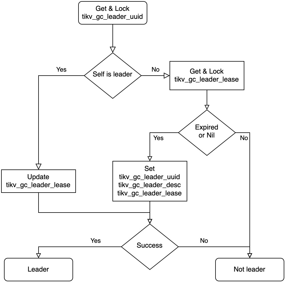
This is the flowchart of leader election which is implemented in checkLeader function, if the result is leader, we then trying to tick a GC.
GC Prepare
When a GC workflow is triggered, we are facing another issue - find out the data that can be cleaned up.
Since TiDB follows SI isolation level, all reads performed in a transaction should get the result from the same timestamp, if not so, there will be consistency and repeatable read issues. Besides, we don't want that the garbage data is cleaned up once after it's not used, because recovery is important when misoperations. That means before starting a GC round, there are many checks.
func (w *GCWorker) checkPrepare(ctx context.Context) (bool, uint64, error) {
	enable, err := w.checkGCEnable()
	...
	now, err := w.getOracleTime()
	...
	ok, err := w.checkGCInterval(now)
	...
	newSafePoint, newSafePointValue, err := w.calcNewSafePoint(ctx, now)
	...
	err = w.saveTime(gcLastRunTimeKey, now)
	...
	err = w.saveTime(gcSafePointKey, *newSafePoint)
	...
	return true, newSafePointValue, nil
}
GC is enabled by default, but it's allowed to be turned off. In prepare stage, it'll check if GC is enabled first.
In TiDB, there is a variable named tikv_gc_run_interval which controls the frequency of GC. It's the min interval between 2 GC rounds, 10min by default.
Once it's ready to perform a GC round, calcNewSafePoint is called to get a new safepoint, this deals with some long-term opened transactions. We'll talk about how safepoint is decided later.
If a new safepoint is got, we then update the GC checkpoint and new safepoint, here we're ready to start a GC round. It's ok that TiDB collapses after the new GC round is set because it won't break the GC promises, we just skip a round of GC.
GC Safepoint
This is the key problem of GC.
What we desired is the min transaction start timestamp between all TiDB instances. TiDB instances will store their min start timestamp in PD's etcd, so we just fetch all the min transaction start timestamps here. GetWithPrefix will get all KV pairs from the etcd storage.
func (w *GCWorker) calcGlobalMinStartTS(ctx context.Context) (uint64, error) {
	kvs, err := w.tikvStore.GetSafePointKV().GetWithPrefix(infosync.ServerMinStartTSPath)
	if err != nil {
		return 0, err
	}

	var globalMinStartTS uint64 = math.MaxUint64
	for _, v := range kvs {
		minStartTS, err := strconv.ParseUint(string(v.Value), 10, 64)
		if err != nil {
			logutil.Logger(ctx).Warn("parse minStartTS failed", zap.Error(err))
			continue
		}
		if minStartTS < globalMinStartTS {
			globalMinStartTS = minStartTS
		}
	}
	return globalMinStartTS, nil
}
TiDB server has the risk of crash, however, if a never-pushed-up min start timestamp is left in the system, GC will never works. To solve this issue, the min start timestamp is set with a lease and if TiDB is offline for a long duration, that min start timestamp will be cleared.
After we get all the min start timestamps from etcd, it's easy to calculate the global min start timestamp. It's easy to know the min start timestamp from a single TiDB instance, and every TiDB instance will report it's min start timestamp to etcd in ReportMinStartTS function every interval.
There is a further situation cannot be handled by calculating the global min start timestamp across all TiDB servers, some tools may require TiDB keep data available for a long time. e.g., when BR is processing backup task, the snapshot should be kept even the specific lifetime has been passed. This is checked when setGCWorkerServiceSafePoint is called.
GC Workflow
Once the safepoint is decided and prepare stage is done, it's ready to start a GC workflow. Generally, there are three steps to do.
- Resolve locks.
- Delete unused ranges.
- GC for every key.
The workflow can be found from GC job function. The main intent of this workflow is to clean up data has more impact on the running tasks earlier.
In resolve locks phase, GC will clean up the locks of aborted transaction and commit the locks of success transaction. GCWorker scans the locks from every store and call BatchResolveLocks for cleaning up, you may read lock resolver chapter for more information about locks.
There are two modes when scanning locks, legacy mode and physical mode. Currently, only legacy mode is stable. The physical mode(a.k.a., Green GC) is introduced in TiDB 4.0, however not GA yet. When it is available, it's possible to scan locks by physical mode which bypasses the Raft layer and scan the locks directly. The resolveLocks function will use legacy mode as a fallback even if physical mode is set.
func (w *GCWorker) resolveLocks(ctx context.Context, safePoint uint64, concurrency int, usePhysical bool) (bool, error) {
	if !usePhysical {
		return false, w.legacyResolveLocks(ctx, safePoint, concurrency)
	}
	// First try resolve locks with physical scan
	err := w.resolveLocksPhysical(ctx, safePoint)
	if err == nil {
		return true, nil
	}
	...
	return false, w.legacyResolveLocks(ctx, safePoint, concurrency)
}
The GCWorker then cleans up unused ranges, which are caused by drop table or drop index statements. When executing the drop statements in TiDB, TiDB only marks some ranges to be deleted and returns success. These to-be-deleted ranges are actually cleaned up in GC.
MySQL [test]> create table t(id int primary key, v int, key k(v));
Query OK, 0 rows affected (0.109 sec)

MySQL [test]> insert into t values(1,1),(2,2),(3,3);
Query OK, 3 rows affected (0.004 sec)
Records: 3  Duplicates: 0  Warnings: 0

MySQL [test]> alter table t drop index k;
Query OK, 0 rows affected (0.274 sec)

MySQL [test]> SELECT HIGH_PRIORITY job_id, element_id, start_key, end_key FROM mysql.gc_delete_range;
+--------+------------+----------------------------------------+----------------------------------------+
| job_id | element_id | start_key                              | end_key                                |
+--------+------------+----------------------------------------+----------------------------------------+
|     58 |          1 | 7480000000000000385f698000000000000001 | 7480000000000000385f698000000000000002 |
+--------+------------+----------------------------------------+----------------------------------------+
1 row in set (0.002 sec)

MySQL [test]> SELECT HIGH_PRIORITY job_id, element_id, start_key, end_key FROM mysql.gc_delete_range_done WHERE 1;
+--------+------------+--------------------+--------------------+
| job_id | element_id | start_key          | end_key            |
+--------+------------+--------------------+--------------------+
|     55 |         53 | 748000000000000035 | 748000000000000036 |
+--------+------------+--------------------+--------------------+
1 row in set (0.002 sec)
The to-be-deleted ranges are stored in mysql.gc_delete_range. They will be deleted in deleteRanges in GC. After they are cleaned up, they will be moved into mysql.gc_delete_range_done, and double-checked after 24 hours.
Finally, the GCWorker is going to clean up the stale keys. From TiDB 5.0, only distributed mode is supported, this document will talk about distributed mode below.
Distributed GC is implemented by pushing up the safepoint in PD. Notice that the safepoint is monotonic. PD guarantees this by comparing the old and new values here.
// UpdateGCSafePoint implements gRPC PDServer.
func (s *Server) UpdateGCSafePoint(ctx context.Context, request *pdpb.UpdateGCSafePointRequest) (*pdpb.UpdateGCSafePointResponse, error) {
	...
	newSafePoint := request.SafePoint

	// Only save the safe point if it's greater than the previous one
	if newSafePoint > oldSafePoint {
		if err := s.storage.SaveGCSafePoint(newSafePoint); err != nil {
			return nil, err
		}
		log.Info("updated gc safe point",
			zap.Uint64("safe-point", newSafePoint))
	} else if newSafePoint < oldSafePoint {
		log.Warn("trying to update gc safe point",
			zap.Uint64("old-safe-point", oldSafePoint),
			zap.Uint64("new-safe-point", newSafePoint))
		newSafePoint = oldSafePoint
	}

	return &pdpb.UpdateGCSafePointResponse{
		Header:       s.header(),
		NewSafePoint: newSafePoint,
	}, nil
}
If PD returns the same new safepoint as TiDB provides, TiDB takes this GC round success.
Distributed GC on TiKV
As we talked above, TiDB only pushes up the safepoint in PD instead of cleaning up keys directly. Every TiKV has an inner GcManager with safe_point field.
#![allow(unused)]
fn main() {
pub(super) struct GcManager<S: GcSafePointProvider, R: RegionInfoProvider, E: KvEngine> {
    cfg: AutoGcConfig<S, R>,

    /// The current safe point. `GcManager` will try to update it periodically. When `safe_point` is
    /// updated, `GCManager` will start to do GC on all regions.
    safe_point: Arc<AtomicU64>,

    safe_point_last_check_time: Instant,

    /// Used to schedule `GcTask`s.
    worker_scheduler: Scheduler<GcTask<E>>,

    /// Holds the running status. It will tell us if `GcManager` should stop working and exit.
    gc_manager_ctx: GcManagerContext,

    cfg_tracker: GcWorkerConfigManager,
    feature_gate: FeatureGate,
}
}
By default, TiKV tries to pull safepoint from PD every 10 seconds. If the pulled safepoint is greater than the local one, the local one will be pushed up, and meanwhile, a GC job is trigger in TiKV locally.
Summary
This document talked about how MVCC GC worked in TiDB system. The most basic requirement of GC is not to delete readable data. Due to the guarantee of GC, you don't need to care about that data is removed. The green GC, skips fetch snapshot when read locks, help to improve the performance of GC. There are some further performance-related topics of GC in TiKV which will be talked in TiKV Dev Guide.
Session
The session package (and related packages such as sessionctx and sessionctx/variable) are responsible for maintaining the state of both sessions and transactions.
New session origins
New connections are first established in the server package. After some initial protocol negotiation, the server package calls session.CreateSession(). This function then calls session.createSessionWithOpt() (via CreateSessionWithOpt()) which creates the session.
Sessions used for internal server operations are usually created in a different manner, with the sessionctx being retrieved from a pool of sessions maintained by domain. For example:
dom := domain.GetDomain(e.ctx)
sysSessionPool := dom.SysSessionPool()
ctx, err := sysSessionPool.Get()
if err != nil {
    return nil, err
}
restrictedCtx := ctx.(sessionctx.Context)
restrictedCtx.GetSessionVars().InRestrictedSQL = true
Internal sessions will not show up in the output of SHOW PROCESSLIST, and skip all privilege checks because they do not have a privilege manager handle attached.
System variable state
System variables follow similar semantics to MySQL:
- If a variable includes
SESSIONscope, the value is copied to the session state when the session is created. - Any changes to the
GLOBALvalue will not apply to any existing sessions.
The state of the variables is stored in sessionVars. The raw string values are stored in a map named systems. This string value is used for persistence in the mysql.global_variables table.
For many variables, as well as a string value there is a typed field in sessionVars. For example:
SessionVars.systems["tidb_skip_utf8_check"] (string) maps to SessionVars.SkipUTF8Check (bool).
The typed value is set when the SetSession attached to the system variable definition is called. For tidb_skip_utf8_check this is as follows:
{Scope: ScopeGlobal | ScopeSession, Name: TiDBSkipUTF8Check, Value: BoolToOnOff(DefSkipUTF8Check), Type: TypeBool, SetSession: func(s *SessionVars, val string) error {
	s.SkipUTF8Check = TiDBOptOn(val)
	return nil
}},
The SetSession function can also be considered an Init function, since it is called when the session is created and the values are copied from global scope. To disable SetSession from being called on creation, skipInit can be set to true. For example with CharsetDatabase:
{Scope: ScopeGlobal | ScopeSession, Name: CharsetDatabase, Value: mysql.DefaultCharset, skipInit: true, Validation: func(vars *SessionVars, normalizedValue string, originalValue string, scope ScopeFlag) (string, error) {
    return checkCharacterSet(normalizedValue, CharsetDatabase)
}, SetSession: func(s *SessionVars, val string) error {
	if cs, err := charset.GetCharsetInfo(val); err == nil {
		s.systems[CollationDatabase] = cs.DefaultCollation
	}
	return nil
}},
In the above example, skipping the SetSession function is useful because it prevents the CollationDatabase from being overwritten when the session is initialized. This is only expected if the user issues a statement to change the CharsetDatabase value.
Differences from MySQL
In TiDB, changes to GLOBAL scoped system variables are propagated to other TiDB servers in the cluster and persist across restarts. The notification event to other servers is sent via an etcd channel in the call domain.GetDomain(s).NotifyUpdateSysVarCache():
// replaceGlobalVariablesTableValue executes restricted sql updates the variable value
// It will then notify the etcd channel that the value has changed.
func (s *session) replaceGlobalVariablesTableValue(ctx context.Context, varName, val string) error {
	stmt, err := s.ParseWithParams(ctx, `REPLACE INTO %n.%n (variable_name, variable_value) VALUES (%?, %?)`, mysql.SystemDB, mysql.GlobalVariablesTable, varName, val)
	if err != nil {
		return err
	}
	_, _, err = s.ExecRestrictedStmt(ctx, stmt)
	domain.GetDomain(s).NotifyUpdateSysVarCache() // <-- the notification happens here
	return err
}
Because GLOBAL scoped variables are propagated to other servers, TiDB also has a special concept of "instance-scoped variables". An instance scoped variable is actually a SESSION scoped variable that has a GetSession method which returns data that is specific to an instance. For example, tidb_general_log:
{Scope: ScopeSession, Name: TiDBGeneralLog, Value: BoolToOnOff(DefTiDBGeneralLog), Type: TypeBool, skipInit: true, SetSession: func(s *SessionVars, val string) error {
	ProcessGeneralLog.Store(TiDBOptOn(val))
	return nil
}, GetSession: func(s *SessionVars) (string, error) {
	return BoolToOnOff(ProcessGeneralLog.Load()), nil
}},
The decision to make an option such as tidb_general_log instance scoped is because it references a file on the local filesystem. This may create issues when global, as the path may not be writable on each tidb-server in the cluster.
As you can see by the Scope: Session, instance-scoped variables are not natively handled by the sysvar framework, but are instead denoted by the GetSession() function reading from a global location. The documentation for tidb_general_log also notes it as "instance" scoped by convention.
Transaction state
The session struct (s.txn) is responsible for keeping modified key-value pairs in a LazyTxn until the transaction commits. A commit statement only sets the session variable state that it is no longer in an active transaction:
func (e *SimpleExec) executeCommit(s *ast.CommitStmt) {
	e.ctx.GetSessionVars().SetInTxn(false)
}
The function autoCommitAfterStmt() which is called as part of finishStmt() is responsible for committing the transaction:
if !sessVars.InTxn() {
	if err := se.CommitTxn(ctx); err != nil {
		if _, ok := sql.(*executor.ExecStmt).StmtNode.(*ast.CommitStmt); ok {
			err = errors.Annotatef(err, "previous statement: %s", se.GetSessionVars().PrevStmt)
		}
		return err
	}
	return nil
}
The session.CommitTxn() function will handle the commit, including retry (if permitted). There is also special handling for both pessimistic and optimistic transactions, as well as removing the key-value pairs which apply to temporary tables from the transaction buffer.
See also
Privilege
At its core, TiDB's approach to user privileges is similar to that of MySQL:
- The privileges are stored in tables such as
mysql.userandmysql.db. - The privilege tables are then loaded into an in-memory cache. The cache is then used by the privilege manager to determine the privileges of a user.
- The cache is automatically updated when using privilege control statements such as
GRANTandREVOKE. The statementFLUSH PRIVILEGEScan also be used to manually reload the cache for when manual changes are made to the privilege tables.
Behavior differences from MySQL
Implicit updates to the privilege cache (i.e. when GRANT or REVOKE statements are executed) run immediately on the instance of TiDB that is executing the statement. A notification is also sent to all TiDB instances to rebuild their cache. This notification is sent asynchronously, so it is possible that when a load balancer is used, the cache will be out of date when attempting to reconnect to a TiDB instance immediately.
Because the asynchronous notifications do not guarantee delivery, TiDB will also automatically rebuild the privilege cache every 5-10 minutes in a loop. This behavior is not strictly MySQL compatible, because in MySQL the privilege cache will only ever be rebuilt from a FLUSH PRIVILEGES statement, a restart, or a privilege control statement.
Client certificate options are stored in the mysql.global_priv table instead of the mysql.user table. This behavior is not intentional, and may be changed in the future.
Adding privilege checks to a statement
Some privilege checks are automatically assigned during plan building, for example ensuring that you have permissions to the tables that will be accessed. These checks are skipped for information_schema tables, and should you add an additional statement (such as SHOW xyz), you will also need to ensure that privilege checks are added.
Should you need to add privilege checks there are two options:
-
During plan building you can attach
visitInfoto the plan (examples:SET CONFIG,SHOW BACKUPS) -
In the executor function which handles the statement (examples:
SHOW PROCESSLIST).
The first option is recommended, as it is much less verbose. However, visitInfo does not handle cases where the statement can behave differently depending on the permissions of the user executing it. All users can execute the SHOW PROCESSLIST statement, but to see the sessions of other users requires the PROCESS privilege.
visitInfo also only supports AND semantics. For complex scenarios (such as DROP USER requiring either CREATE USER OR DELETE privileges on the mysql.user table), option 2 is required.
Manually checking with the privilege manager
For (2) above, manual checks should follow the following pattern:
checker := privilege.GetPrivilegeManager(e.ctx)
if checker != nil && !checker.RequestVerification(ctx.GetSessionVars().ActiveRoles, schema.Name.L, table.Name.L, "", mysql.AllPrivMask) {
    /* do something */
}
..
if checker == nil || !checker.RequestDynamicVerification(ctx.GetSessionVars().ActiveRoles, "RESTRICTED_TABLES_ADMIN", false) {
    /* do something */
}
The check for checker != nil is important because for internal SQL statements the privilege manager is not present. These statements are expected to fall through and satisfy the privilege check.
Static and dynamic privileges
Privileges fall into two categories:
- Static privileges: These are the "traditional" privileges such as
INSERT,UPDATE,SELECT,DELETE,SUPER,PROCESSwhich have existed in MySQL for a long time. They can usually be assigned to a user on either a global or database/table level. - Dynamic privileges: These are new privileges such as
BACKUP_ADMIN,RESTORE_ADMIN,CONNECTION_ADMIN. They can only be assigned on a global level, and each have their own "grantable" attribute.
Dynamic privileges were introduced in MySQL 8.0 (and TiDB 5.1) to solve a specific issue, which is that the SUPER privilege is too coarse. There are many scenarios where a user needs to be assigned the SUPER privilege to perform a specific action, but too many other privileges are granted at the same time.
Any statements added to TiDB should no longer require the SUPER privilege directly. Instead, a dynamic privilege should be added which will be satified by the SUPER privilege.
Security Enhanced Mode
TiDB features an extension to MySQL called Security Enhanced Mode (SEM), which is disabled by default. One of the main aims of SEM is to reduce the privileges of SUPER and instead require specific "restricted" dynamic privileges instead. The design is inspired by features such as "Security Enhanced Linux" (SeLinux) and AppArmor.
SEM plugs directly into the privilege manager, but the hard coded list of restricted objects lives in ./util/sem/*. It is expected that over time SEM will protect against additional operations which are considered to be high risk or too broad.
Recommended Reading
- Technical Design: Security Enhanced Mode
- Technical Design: Dynamic Privileges
- MySQL Worklog: Pluggable Dynamic Privileges
Plugin
The plugin API allows TiDB to be extended with new features such as audit logging or IP allow/deny listing.
Sample code is provided for a basic audit logging plugin at plugin/conn_ip_example/. For an example on compiling TiDB and this plugin:
plugin="conn_ip_example"
cd cmd/pluginpkg
go install
cd ../../plugin/$plugin
pluginpkg -pkg-dir . -out-dir .
cd ../..

./bin/tidb-server -plugin-dir plugin/$plugin -plugin-load $plugin-1
An explanation of what this does:
cd cmd/pluginpkgandgo installcompiles the command line utility calledpluginpkg, which is used to build the plugin.pluginpkg -pkg-dir . -out-dir .reads the plugin code +manifest.tomlfile and generates a shared object file for the plugin (conn_ip_example-1.so).- When the tidb-server starts, it can load plugins in a specified directory (
plugin-dir).
You can confirm which plugins are installed with the SHOW PLUGINS statement:
mysql> show plugins;
+-----------------+--------------+-------+--------------------------------------------------------------------------------------+---------+---------+
| Name            | Status       | Type  | Library                                                                              | License | Version |
+-----------------+--------------+-------+--------------------------------------------------------------------------------------+---------+---------+
| conn_ip_example | Ready-enable | Audit | /home/morgo/go/src/github.com/morgo/tidb/plugin/conn_ip_example/conn_ip_example-1.so |         | 1       |
+-----------------+--------------+-------+--------------------------------------------------------------------------------------+---------+---------+
1 row in set (0.00 sec)
Customizing the example plugin
The manifest file describes the capabilities of the plugin, and which features it implements. For a basic version:
name = "conn_ip_example"
kind = "Audit"
description = "just a test"
version = "1"
license = "" # Suggested: APLv2 or GPLv3. See https://choosealicense.com/ for details
validate = "Validate"
onInit = "OnInit"
onShutdown = "OnShutdown"
export = [
    {extPoint="OnGeneralEvent", impl="OnGeneralEvent"},
    {extPoint="OnConnectionEvent", impl="OnConnectionEvent"}
]
In addition to this basic example, plugins can also implement an OnFlush function. This is called when the statement FLUSH TIDB PLUGINS pluginName is executed. TiDB does not require plugins to implement a OnFlush function, but when specified it will call this method on all TiDB nodes in the cluster.
OnConnectionEvent
The OnConnectionEvent is called when a new connection is initially created (event plugin.ConnectionEvent == plugin.PreAuth) and again when the connection is successfully established (event plugin.ConnectionEvent == plugin.Connected).
To prevent a connection from being created, an error should be returned for the event plugin.PreAuth.
OnGeneralEvent
The OnGeneralEvent is called:
- Before a statement starts execution (
event plugin.GeneralEvent == plugin.Starting) - Ater a statement has completed execution (
event plugin.GeneralEvent == plugin.Completed)
General events are useful for auditing operations performed by users. Because sctx SessionVars is available in the OnGeneralEvent function, it is possible to obtain a lot of additional information about the statement being executed. For example:
sctx.Usercontains the*auth.UserIdentityof the user who is executing this session, andsctx.ActiveRolescontains the list of active roles associated with the session.sctx.DBNamecontains the name of the database the user is executing in.sctx.StmtCtxcontains the context of the statement that was executed. For examplesctx.StmtCtx.SQLDigest()can be called to get a digest of the executed statement, andsctx.StmtCtx.Tablescontains a slice of tables that are accessed by the statement.
The current implementation of OnGeneralEvent does not permit errors to be returned. It is possible that this may change in a future version, since this will allow pre-execution checks to be performed on statements.
Additional Reading
System tables
There are multiple types of system tables:
mysqlschema: There are mostly real tables stored on TiKVinformation_schema: These tables are generated on request and not stored on disk.performance_schema: These tables are generated on request and not stored on disk.metrics_schema: These are metrics from Prometheus, not real tables.SYS: these are views etc to makeperformance_schemaeasier to use.
See also the docs:
- TiDB mysql schema
- TiDB information_schema
- TiDB performance_schema
- TiDB sys schema
- TiDB metrics_schema
- MySQL performance_schema
- MySQL information_schema
- MySQL sys schema
- MySQL mysql schema
information_schema
slow_query
Overview
Slow queries logs are written to tidb-slow.log (set with slow-query-file in the config) if they are over the slow-threshold (300ms by default). If record-plan-in-slow-log is enabled this will include the execution plan. This uses slowLogEncoder.
Each TiDB node writes its own slow logs.
SLOW_QUERY
   +------------+
   | App or CLI |
   +------------+
         |
     SQL Query
     SLOW_QUERY
         |
     +--------+
     |  TiDB  |
     +--------+
         |
  +---------------+
  | tidb-slow.log |
  +---------------+
The slow log can be viewed directly or via the information_schema.SLOW_QUERY table.
The column definition is in slowQueryCols.
The SlowQueryExtractor helps to extract some predicates of slow_query.
A lot of the other logic can be found in slow_query.go.
This table has RuntimeStats, which adds stats to EXPLAIN ANALYZE output.
CLUSTER_SLOW_QUERY
There is also the information_schema.CLUSTER_SLOW_QUERY table that combines the slow log from all nodes into a single table.
The TiDB Dashboard uses the CLUSTER_SLOW_QUERY table to display the slow queries in a webpage.
                  +----------------+
                  | TiDB Dashboard |
                  |   or App/CLI   |
                  +----------------+
                         |
                      SQL Query
                  CLUSTER_SLOW_QUERY
                         |
                      +--------+
        +--gRPC-------| TiDB 1 |------gRPC--+
        |             +--------+            |
   +--------+            |               +--------+
   | TiDB 0 |            |               | TiDB 2 |
   +--------+            |               +--------+
      |                  |                  |
+---------------+  +---------------+  +---------------+
| tidb-slow.log |  | tidb-slow.log |  | tidb-slow.log |
+---------------+  +---------------+  +---------------+
CLUSTER_SLOW_QUERY is using the coprocessor gRPC interface to send cop requests to the TiDB node. This allows the reuse of query condition push down and column prune, to reduce unnecessary data transfer.
There are no RuntimeStats for this table, see this issue for a request to add that.
Documentation
Project Management
Practices for managing the TiDB project:
Release Train Model
What is the release train model?
Before introducing the concept of the release train model, let us take a review of the delivery mode of TiDB in the past.
In releases earlier than v5.0, the release frequency of TiDB major versions was a year or half a year, which is quite a long development cycle. The long development cycle has both benefits and drawbacks as follows:
- Benefits: the longer a development cycle is, the more features one release can deliver.
- Drawbacks: the longer a development cycle is, the more difficulties we have to coordinate regression and acceptance tests, and the more possibly a delay happens. Also, if new feature requests are received during the long development cycle, these new features are added to the development backlog after the start of the development cycle. In this case, development tasks are hardly converged before the release date.
Starting from v5.0, TiDB adopts the release train model, which is a product development model for requirements gathering, analysis, decision making, release, and issue feedback.
Just like a train delivering goods, decisions need to be made about the priorities of the goods, destination, arrival time, which train to load on, which carriage, etc., before the train departs.
The benefits of moving to the release train model are as follows:
- A shorter feedback cycle: users can benefit from features shipped faster.
- Easier predictability for contributors and users:
- Developers and reviewers can decide in advance the target release to deliver specific features.
- If a feature misses a release train, we have a good idea of when the feature will show up later.
- Users know when to expect their features.
- Transparency. There will be a published cut-off date (AKA code freeze) for the release and people will know about the date in advance. Hopefully this will remove the contention around which features will be included in the release.
- Quality. we've seen issues pop up in release candidates due to last-minute features that didn't have proper time to bake in. More time between code freeze and release will let us test more, document more and resolve more issues.
- Project visibility and activity. Having frequent releases improves our visibility and gives the community more opportunities to talk about TiDB.
Because nothing is ever perfect, the release train model has some downsides as well:
- Most notably, for features that miss the code-freeze date for a release, we have to wait for a few months to catch the next release train. Most features will reach users faster as per benefit #1, but it is possible that a few features missing the code-freeze date might lose out.
- With the frequent releases, users need to figure out which release to use. Also, having frequent new releases to upgrade may be a bit confusing.
- Frequent releases means more branches. To fix a bug of an old release, we need to work on more old branches.
We decided to experiment with release train model and see if the benefits for us as a community exceed the drawbacks.
How will TiDB development process look like?
At this stage we are planning to make a release every two months.
Thus, a typical development cycle takes two months, which we call a sprint. For example, the development cycle of v5.2 is from the end of June to the end of August and is called Sprint 4.
Two weeks before the release date, the release manager will create a branch for the new release based on the master branch, publish a list of features to be included in the release, and also announce the code-freeze, after which only fixes for blocking bugs can be merged.
For the release train model, we strictly ensure that a release happens on the planned date. For example, we decide to deliver the v5.2 release by the end of August so we will stick to it. If any features cannot be completed by the code-freeze date, we will drop them and avoid taking them into the new release branch. In this case, the development in the master branch can still work as usual and those features will be moved to the following release.
Ideally, we would have started stabilization once we create the new release branch. After the code-freeze date, only pull requests of blocker bugs can be merged to the new release branch. In a rare scenario, it is possible that few features pass the code freeze bar but still fail to be completed on time. Such features will also be dropped from the release train in the end to meet the release deadline.
Developers who want to contribute features to TiDB could follow the procedure described in Make a Proposal. Once all the requirements are met and all the codes are merged into the master branch, the feature will be boxed into the nearest release.
Except for feature releases, there also exists patch releases. Patch releases are scheduled when needed, there is no fixed calendar for such releases. When a patch release is scheduled, there are two rounds of triage. A bug fix could only be boxed into a release when it occurs before triage. Get more information about TiDB releases and versions in TiDB versioning.
What happens if features are not completed?
Different features have different complexities. Some features can be implemented within a single release while some features span multiple releases. There are two conventional development strategies:
-
Ensure that each feature is split into testable units and only testable units get merged. This means that a good set of unit tests and system tests are written for sub-tasks before they are merged. This approach ensures that the master branch is in a relatively stable state and can be released at any time.
-
Use feature branches. For a specific feature, the feature developers create a branch from the master branch and ensure that the branch is in sync with the master branch from time to time. Only when the feature developers and reviewers have a high level of confidence in the feature stability, the feature can be merged into master. This approach brings the additional overhead of branching and performing merges from time to time.
With the release train model, to ensure that ongoing features do not affect the stability of the release, TiDB chooses feature branches strategy.
Support Phases
For definitions of release types (LTS, DMR, patch), see TiDB Versioning. Each LTS release goes through these support phases:
- Maintenance Support: Regular patch releases address reported issues and security vulnerabilities.
- Extended Support: One additional year of critical security patches only.
- End of Life (EOL): No further support is provided.
Community edition and enterprise edition timelines may differ. The TiDB Release Support Policy is the authoritative reference for current support dates.
Current Maintained Releases
The community edition support dates below are sourced from the TiDB Release Support Policy, which is the authoritative reference. Refer to that page for enterprise edition timelines and any updates.
| version | branch | status | triage label | latest release | community edition support until | issue |
|---|---|---|---|---|---|---|
| v8.5 | release-8.5 | LTS | affects-8.5 | v8.5.6 | 2027-12-19 | https://github.com/pingcap/tidb/issues/65584 |
| v8.1 | release-8.1 | LTS | affects-8.1 | v8.1.2 | 2027-05-24 | https://github.com/pingcap/tidb/issues/58699 |
| v7.5 | release-7.5 | LTS | affects-7.5 | v7.5.7 | 2026-12-01 | https://github.com/pingcap/tidb/issues/60574 |
| v7.1 | release-7.1 | LTS | affects-7.1 | v7.1.6 | 2026-05-31 | https://github.com/pingcap/tidb/issues/57028 |
| v6.5 | release-6.5 | LTS | affects-6.5 | v6.5.12 | 2025-12-29 | https://github.com/pingcap/tidb/issues/59101 |
| v6.1 | release-6.1 | LTS | affects-6.1 | v6.1.7 | 2025-06-13 | https://github.com/pingcap/tidb/issues/42918 |
For more versions' information, please check https://github.com/pingcap/tidb/projects/63.
TiDB Versioning
TiDB versioning has the form X.Y.Z where X.Y refers to the release series and Z refers to the patch number. Starting with TiDB 6.0, TiDB is released as two different release series:
- LTS(Long-Term Support) Releases
- DMR(Development Milestone) Releases
LTS Releases
LTS releases are made available approximately every six months. They carry new features and improvements and are recommended to deploy into production environments. There will be patch releases based on the LTS releases in their lifecycle. Example versions:
5.46.1
Release 4.0 and 5.x are treated like LTS releases although they are earlier than 6.0.
DMR Releases
DMR releases are made available approximately every two months. Every 3rd DMR release turns into a LTS release. Same as LTS releases, a DMR release introduces new features and improvements. But there is no patch releases based on the DMR release. Bugs in the DMR release are going to be fixed in the next DMR/LTS releases. There is a -DMR suffix of DMR versioning. Example versions:
6.0.0-DMR6.2.0-DMR
Patch Releases
Patch releases generally include bug fixes for LTS releases. There is no fixed release schedule for patch releases. Example versions:
6.1.16.1.2
Historical Versioning
There are some other versioning in history which are not used any more.
GA(General Availability) Releases
Stable release series, released after RC releases. GA releases are recommended for production usage. Example versions:
2.1 GA5.0 GA
RC(Release Candidate) Releases
RC releases introduces new features and improvements and meant for early test. Comparing with Beta releases, RC releases are much more stable and suitable for test, but not suitable for production usage. Example versions:
2.0-RC13.0.0-rc.1
Beta Releases
Beta releases introduces new features and improvements. Comparing with Alpha releases, Beta releases shall not carry any critical bugs. Early adopters could use Beta releases to try new features. Example versions:
1.1 Beta4.0.0-beta.1
Alpha Releases
The very first releases in a series. Used for fundamental functionality and performance test. Example versions:
1.1 Alpha
Extending TiDB
Add a function
To add a builtin function to TiDB the best practice is to look at MySQL first and try to implement the function in such a way that it is commpatible. Avoid adding functions that are already deprecated in MySQL or that might soon be deprecrated.
Here we will implement a HELLO() function that has one argument that is a string. For this you need a clone of the pingcap/tidb repository
sql> SELECT HELLO("world");
ERROR: 1305 (42000): FUNCTION test.hello does not exist
The first step is to define the name of the function in parser/ast/functions.go:
// List scalar function names.
const (
...
        Hello = "hello"
)
This links ast.Hello with "hello". Note that the lookup for the function is done with the lowercase name, so always use the lowercase name, otherwise it won't find the function.
The next step is to modify expression/builtin.go
var funcs = map[string]functionClass{
...
        ast.Hello: &helloFunctionClass{baseFunctionClass{ast.Hello, 1, 1}},
}
Now we need to define helloFunctionClass. We will do this in expression/builtin_string.go. The functions are organised in multiple files, pick the one that fits best.
var (
...
        _ functionClass = &helloFunctionClass{}
)
...
var (
        _ builtinFunc = &builtinHelloSig{}
)
...
type helloFunctionClass struct {
        baseFunctionClass
}

func (c *helloFunctionClass) getFunction(ctx BuildContext, args []Expression) (builtinFunc, error) {
        if err := c.verifyArgs(args); err != nil {
                return nil, err
        }
        bf, err := newBaseBuiltinFuncWithTp(ctx, c.funcName, args, types.ETString, types.ETString)
        if err != nil {
                return nil, err
        }
        sig := &builtinHelloSig{bf}
        return sig, nil
}

type builtinHelloSig struct {
        baseBuiltinFunc
}

func (b *builtinHelloSig) Clone() builtinFunc {
        newSig := &builtinHelloSig{}
        newSig.cloneFrom(&b.baseBuiltinFunc)
        return newSig
}

func (b *builtinHelloSig) evalString(ctx EvalContext, row chunk.Row) (name string, isNull bool, err error) {
        name, isNull, err = b.args[0].EvalString(ctx, row)
        if isNull || err != nil {
                return name, isNull, err
        }
        return "hello " + name, false, nil
}
The getFunction() method can return different functions depending on the type and number of arguments. This example always returns the same function that has one string argument and returns a string.
Here evalString() gets called for every row. If the function returns an integer you have to use evalInt and there are also functions for Decimal, Real, Time and JSON.
Now you need to build TiDB again and try the newly added function.
The final result:
sql> SELECT HELLO("world");
+----------------+
| HELLO("world") |
+----------------+
| hello world    |
+----------------+
1 row in set (0.0007 sec)
To show the function with multiple rows:
sql> WITH names AS (SELECT "Europe" AS "name" UNION ALL SELECT "America" UNION ALL SELECT "China")
   -> SELECT HELLO(name) FROM names;
+---------------+
| HELLO(name)   |
+---------------+
| hello Europe  |
| hello America |
| hello China   |
+---------------+
3 rows in set (0.0008 sec)
For testing have a look at expression/builtin_string_test.go.